Table of Contents
Introduction – Excel FILTER Function
The Filter function in Excel 365/2021 is one of the best alternatives to the conventional filtering methods (Auto Filter & Advanced Filter). Once you apply the filter using Filter function in Excel, you don’t need to worry about the data changes. Excel handles everything automatically and recalculate the formula and show the result on latest available data.
Availability of FILTER Function in Excel
Filter Function is available in Excel for Microsoft 365, Excel for Microsoft 365 for Mac, Excel for the web, Excel 2021, Excel 2021 for Mac, Excel 2019, Excel for iPad, Excel for iPhone, Excel for Android tablets, and Excel for Android phones.

Excel Filter Function Definition & Syntax
The FILTER function in Excel 365 allows us to filter a range of data based on a Boolean (True/False) array provided as a parameter in function. Here, Boolean array works like criteria to filter the data.
Note:
Filter function belongs to the category of Dynamic Array function family where the result is array of the values which spills into a range of cells.
A Boolean array is a sequence of values that can only hold the values of true or false i.e. Boolean data type.
Syntax of Filter function in Excel
=FILTER (array, include, [if_empty])
Parameters & description:
- Array (mandatory) – the array or range of cells that you want to filter.
- Include (mandatory) – this is the criteria supplied to filter function as Boolean array (True/False). While executing the formula, Filter function checks the criteria and match it with the value available in respective cell. If the given criteria meets, then It shows True otherwise False in Boolean array and then filters only those records where value is True.
Note: The height (when data is in columns) or width (when data is in rows) of Boolean array (include parameter) must be equal to the height/width of the array argument values of true or false i.e. Boolean data type.
- If_empty (optional) – the value to return if all values in the included array are empty (filter does not return anything).
Notes:
- Array is a range of cells available in a row, a column or a combination of rows and columns of values in Excel. Example, range A2:A5, A2:G2 or A2:G5.
- The Filter function returns the output as an array, which spills the result of the formula in dynamically created appropriate sized array range.
- If you think that the result of Filter could be empty value, then use the 3rd argument ([if_empty]). Otherwise, a #CALC! error will be the result as Excel does not support empty arrays.
- If any value of the Boolean array (include argument) is an error value e.g., #N/A, #Value, etc. or the given condition can’t be converted to a Boolean then Filter function will return an error as output.
- If Array is available in different workbook and you are using Filter function in other workbook, then both workbooks must be opened at the same time. If you close the source workbook, then Filter function will return a #REF! error when it will be refreshed.
How to use the FILTER function in Excel
To understand the different usages of the Filter function in Excel, we will use the below table.
| City | State | Country |
| Bengaluru | Karnataka | India |
| Mangaluru | Karnataka | India |
| Hubli | Karnataka | India |
| Ballari | Karnataka | India |
| Hassan | Karnataka | India |
| Udupi | Karnataka | India |
| Mumbai | Maharashtra | India |
| Pune | Maharashtra | India |
| Nagpur | Maharashtra | India |
| Thane | Maharashtra | India |
| Nasik | Maharashtra | India |
| Aurangabad | Maharashtra | India |
| Peshawar | Khyber Pakhtunkhwa | Pakistan |
| Mardan | Khyber Pakhtunkhwa | Pakistan |
| Mingora | Khyber Pakhtunkhwa | Pakistan |
| Kohat | Khyber Pakhtunkhwa | Pakistan |
| Karachi | Sind | Pakistan |
| Sukkur | Sind | Pakistan |
| Larkana | Sind | Pakistan |
| Huntsville | Alabama | United States |
| Monroe | Louisiana | United States |
| Raleigh | North Carolina | United States |
| Jacksonville | Florida | United States |
| Los Angeles | California | United States |
| Cranston | Rhode Island | United States |
| Milwaukee | Wisconsin | United States |
| Virginia Beach | Virginia | United States |
| New York City | New York | United States |
| Louisville | Kentucky | United States |
Basic Filter function
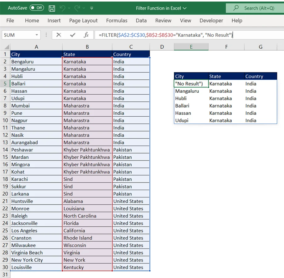
In the following example, we have used the formula =FILTER ($A$2:$C$30, $B$2:$B$30=”Karnataka”, “No Result”) to return all the records for Karnataka as state available in source data (array). If there are no records for Karnataka, then function will return a string “No Result”.
Unlike Auto Filter/Advanced Filter features in Excel, the Filter Function does not make any changes to the source data. It filters the records basis the condition passed to the Include parameter and spill the result array into the range (E5:G10 in the screenshot below), beginning in the cell where the formula is entered.
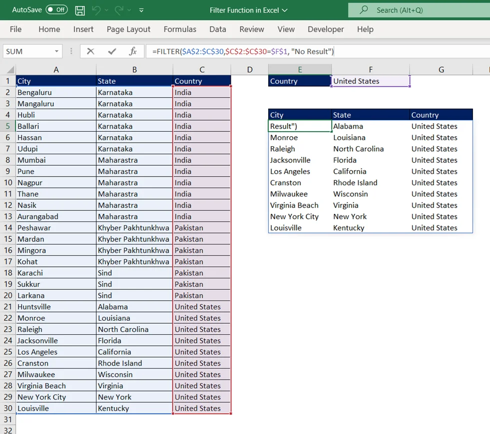
In the above example, we have passed a string value ‘Karnataka’ to the second parameter ‘Include’. You can also pass the cell reference in place of string. Please see the below formula where we are filtering the county ‘United States’.
=FILTER($A$2:$C$30,$C$2:$C$30=$J$1, “No Result”)
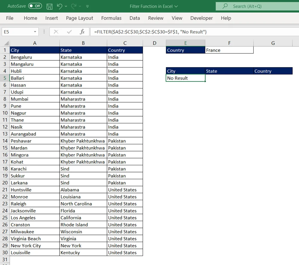
If the given condition (in Include parameter) does not find any records in source data (array) then, the Filter function returns the value we have passed to the last parameter if_empty. In our example, we have passed “No Result” hence, Filter function will show No Result as output of formula.
Please see the below example where we are looking for country as a France but in source data, France is not available. So, the output would be ‘No Result’.
=FILTER($A$2:$C$30,$C$2:$C$30=$F$1, “No Result”)
Here, in place of “No Result”, you can also use an empty string (“”) for the last argument if_empty.
Filter Function in Excel for horizontally structured data table/source
If our data table is horizontally structured unlike vertical in previous examples, then Filter function in Excel also works without any issue. All the conditions and rules will remain same as Vertical table except the width of Boolean array passed as a parameter for Include should have same width of Array, the first argument.
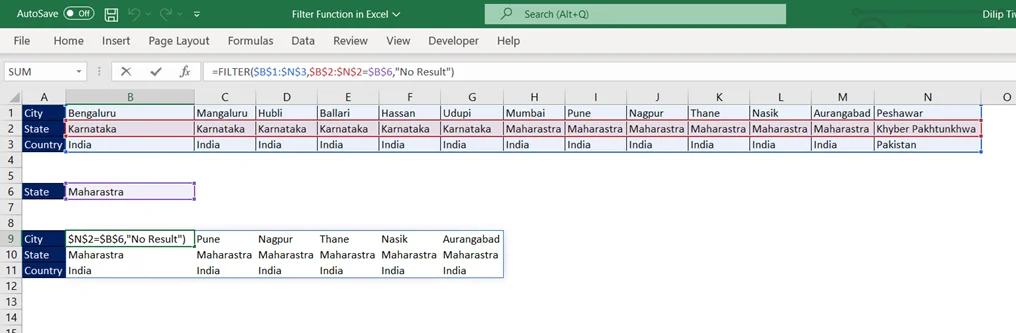
Please see the below example where data is organized horizontally from left to right and we are using Filter function in Excel to get the records where State is Maharashtra.
=FILTER($B$1:$N$3,$B$2:$N$2=$B$6,”No Result”)
Advanced use of Filter function in Excel
In previous example, we have seen the Filter function with simple condition. Let’s understand how we can pass multiple criteria in Filter function.
How To Use Excel FILTER Function with Multiple Criteria Using AND Logic
To filter data with multiple conditions, we can use two or more Boolean arrays with valid Boolean operator (* and +) for the Include parameter.
Before writing the Filter function with AND logic, let’s understand the Boolean arrays for Include parameter in multiple criteria.
As we know, Filter function converts Include parameter value to True and False basis the criteria and then it shows the records having True value only. The same process happens with multiple criteria too, but the condition is all the multiple criteria should get converted into a single Boolean array, where TRUE equates to 1 and FALSE to 0.
So, if we are using two Boolean arrays for the Include parameter then we can use asterisk (*) to multiply the result of first Boolean array value (True and False) to the second Boolean array value and get a single i.e., the final Boolean array (1 and 0) for Filter function. Final Boolean array result will be based on the below Boolean calculation logic.
| TRUE | X | TRUE | = | TRUE |
| TRUE | X | FALSE | = | FALSE |
So, considering the calculation logic, asterisk (*) will be used as AND operator in multiple criterial in Filter function.
| Boolean Value -1 | Boolean Value – 2 | Final Boolean Value |
| TRUE | TRUE | 1 |
| FALSE | FALSE | 0 |
| TRUE | TRUE | 1 |
| TRUE | FALSE | 0 |
| FALSE | FALSE | 0 |
| FALSE | FALSE | 0 |
| FALSE | TRUE | 0 |
| TRUE | TRUE | 1 |
| TRUE | TRUE | 1 |
Let’s apply the same logic to pass multiple filter criteria with AND Boolean operator.
In below formula, we are applying Filter function to get the records where country is India and state is Karnataka.
=FILTER($A$2:$C$30,($C$2:$C$30=$F$1)*($B$2:$B$30=$F$2), “No Result”)

How To Use Excel FILTER Function with Multiple Criteria Using OR Logic
OR logic with multiple criteria is totally different than AND. Unlike AND, either of any criteria will have TRUE value from multiple Boolean arrays then the final Boolean array value will be TRUE.
So, if we are using two Boolean arrays for the Include parameter then we can use plus (+) to sum the result of first Boolean array value (True and False) and the second Boolean array value and get a single i.e., the final Boolean array (True and False) for Filter function. Final Boolean array result will be based on the below Boolean calculation logic for OR.
| TRUE | + | TRUE | = | TRUE |
| TRUE | + | FALSE | = | TRUE |
| FALSE | + | FALSE | = | FALSE |
Let’s apply the same logic to pass multiple filter criteria with OR Boolean operator.
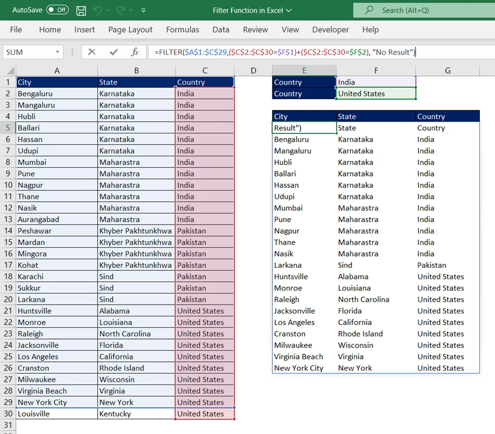
In below formula, we are applying Filter function to get the records where country is either India or United States.
=FILTER($A$1:$C$29,($C$2:$C$30=$F$1)+($C$2:$C$30=$F$2), “No Result”)
How To Use Excel FILTER Function with Multiple Criteria Using AND & OR Logic Both
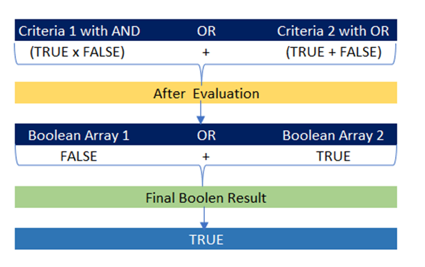
In previous two examples, we have seen the Filter function usage on multiple criteria using AND & OR separately. Let us understand how we can use AND & OR both in multiple criteria of Filter function. The Boolean calculation logic for AND & OR will remain same as we have seen in previous example. The final True and False value will be based on the criteria grouped with brackets ().
So, if multiple criteria for OR has been grouped in one bracket then Filter function in Excel will execute the grouped criteria for OR and convert it to a new Boolean array and after that it executes the AND criteria similar to OR and create an additional new Boolean array and then finally evaluate the criteria with available AND/OR.
Please see the calculation logic as mentioned below.
Let us apply the same logic to pass multiple filter criteria with AND & OR both Boolean operators.
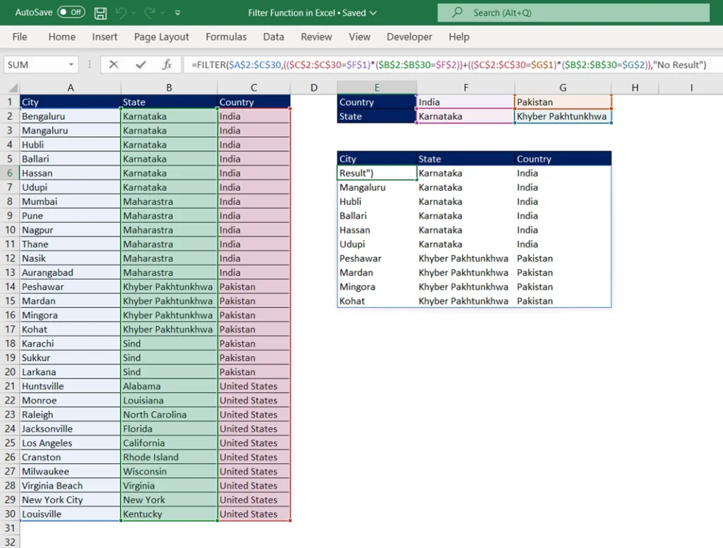
In below formula, we are applying Filter function to get the records where country is India and state is Karnataka or country is Pakistan and state is Khyber Pakhtunkhwa.
=FILTER($A$2:$C$30,(($C$2:$C$30=$F$1)*($B$2:$B$30=$F$2))+(($C$2:$C$30=$G$1)*($B$2:$B$30=$G$2)),”No Result”)
Excel FILTER Function on Numeric or Date Range
In all the above example, we have considered the criteria as string value. You can use any numeric value range or date range for Boolean array and apply the criteria with below mentioned comparison.
| Comparison Operator | Remarks |
| > | Greater Than |
| < | Less Than |
| >= | Greater Than or Equal To |
| <= | Less Than or Equal To |
| <> | Not Equal To |
| = | Equal To |
To understand this, let’s take the sales data with Order Date and Sales amount column.
| Order Date | Customer Name | Sales Amount |
| 1-Jun-22 | Aadi Srivastava | $ 261.96 |
| 2-Jun-22 | Aadi Srivastava | $ 731.94 |
| 3-Jun-22 | Aarav Arya | $ 14.62 |
| 4-Jun-22 | Aarnav Gupta | $ 957.58 |
| 5-Jun-22 | Aarnav Gupta | $ 22.37 |
| 9-Jun-22 | Aayush Kumar | $ 15.55 |
| 10-Jun-22 | Abdul Kumar | $ 407.98 |
| 12-Jun-22 | Abeer Kumar | $ 2.54 |
| 13-Jun-22 | Abhimanyu Kumar | $ 665.88 |
| 14-Jun-22 | Abhiram Pandey | $ 55.50 |
| 15-Jun-22 | Aditya Arya | $ 8.56 |
| 16-Jun-22 | Aditya Arya | $ 213.48 |
| 17-Jun-22 | Aditya Arya | $ 22.72 |
| 18-Jun-22 | Advaith Pandey | $ 19.46 |
| 20-Jun-22 | Advay Srivastava | $ 71.37 |
| 21-Jun-22 | Advik Gupta | $ 1,044.63 |
| 22-Jun-22 | Agastya Gupta | $ 11.65 |
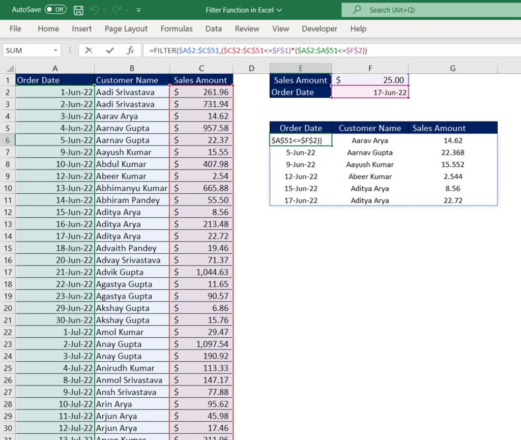
In below formula, we are applying Filter function in Excel to get the records where Order Date is less than or equal to 17th June 2022 and Sales Amount is less than or equal to $25.
=FILTER($A$2:$C$51,($C$2:$C$51<=$F$1)*($A$2:$A$51<=$F$2))
Excel FILTER function – miscellaneous scenario
How to filter duplicates in Excel
If you want to filter duplicate records, then you can leverage the COUNTIFS function and used in FILTER to get the desired output. Just apply the FILTER function as mentioned below.
=FILTER (array, COUNTIFS (column1, column1, column2, column2)>1, “No results”)
Here, we are using all column in COUNTIFS function. If you want to avoid multiple column in COUNTIFS function then you can create a Key column.
How to filter out blanks in Excel
If you want to filter all the records having at least one blank value, then you can use the below mentioned FILTER function to filter out the blank value.
=FILTER(array, (column1<>””) * (column2=<>””), “No results”)
In above formulas, to identify non-blank cells, we have used “not equal to” operator (<>) together with an empty string (“”) to filter out the records with blank value for at least one column.
How to use FILTER function in place of SUMIFS, AVERAGEIFS, COUNTIFS, MINIFS, MAXIFS, etc.?
Using FILTER in place of SUMIF/SUMIFS
=SUM(FILTER (Array, Boolean_array=criteria, “No results”))
Here, Array is a single dimension array (one column/row range) with numerical data which can be summarized and Boolean_array is the array on which we need to apply the criteria. Once, FILTER function will show the result then sum will provide the sum of output array.
Using FILTER in place of AVERAGEIFS/AVERAGEIF
=AVERAGE (FILTER (Array, Boolean_array=criteria, “No results”))
Using FILTER in place of COUNTIFS/COUNTIF
=COUNT (FILTER (Array, Boolean_array=criteria, “No results”))
You can use the same logic for other functions e.g., MAXIFS, MINIFS, etc. …
We can use the FILTER function in different scenarios. Using other Excel functions, you can extend the power of FILTER function.
If you have any questions or need support on this function, then please post your comments related with Filter function in Excel and we will get back to you.
Please download the Excel file used for Filter Function in Excel demo from the below link.


