In this article, we will discuss how to create a chart and change the series & it’s value on mouse hover. Though, there is no Mouse Hover event in Excel however, we will use an alternate method to simulate Mouse Hover event and change the series of a line chart. You can apply the same tips for other charts or calculation in Excel.
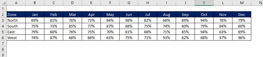
Below is the snapshot of data which has been used in this chart. This is the zone-wise sales performance data from Jan to Dec.
Have created a support table for line chart.

Insert a line chart on the support table and format the chart and move to first worksheet.
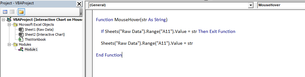
Jump to visual basic application window and insert a blank module. Create a User Defined function.
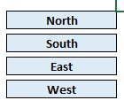
Now, move to Excel window and create labels for North, South, East and West.
User the Hyperlink formula and pass the user-defined function as a parameter in Hyperlink function. Refer the below mentioned formula for North. Replicate the same for other zone as well.
=”North” & IFERROR(HYPERLINK(MouseHover(“North”),””),””)
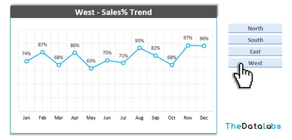
Now, our interactive chart is done.
Please watch this step by step tutorial on YouTube.
Please click on below button to download the excel file used in this tutorial.