How to develop animated Countdown Timer in Excel?
Microsoft Excel provides a lot of flexibilities to modify charts and make several eye-catching visualizations and utility tools. Countdown timer is one of the best examples of that. MS Excel based Countdown Timer is a simple, easy to use, and free of cost to develop. With Countdown Timer, you can track time in Excel without installing any applications or visiting to any website. TheDataLabs Team has developed this tool with the help of Pie and Doughnut Chart. Animation effect has been added with VBA code. If you are familiar with basic charts and macro, then you can easily create this beautiful utility tool within 10 to 15 minutes.

Follow the below steps to create this awesome utility tool from scratch.
1.Open Excel Application
2.Create a Blank Workbook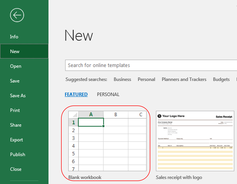
3.Save the Workbook as ‘Countdown Timer.xlsm’
4.Rename the ‘Sheet1’ to ‘CountDown Timer’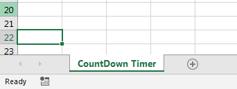
5.Un-check the ‘Gridlines’ under ‘Show’ group in ‘View’ tab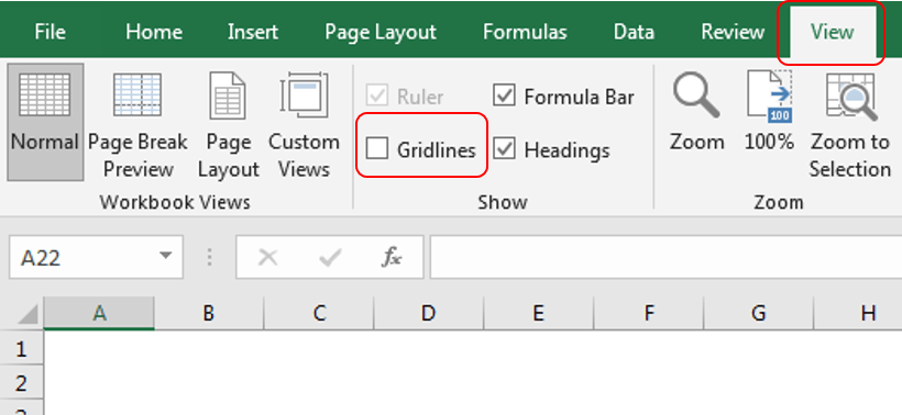
6.Prepare input tables for User input, Pie Chart and Doughnut Chart. Follow the below picture to create all the required tables
7.Enter the values in first two highlighted tables (Doughnut and Pie Chart). Please use the values available in below image and update the table accordingly.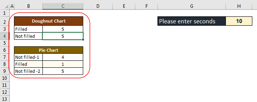
8.Select the Range C3:C4 in Doughnut Chart table. Go to Insert tab, click on Pie Chart and select Doughnut Chart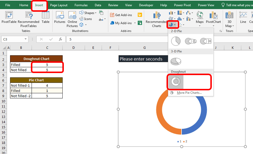
9.Select the Doughnut Chart, go to Format tab and change the Size: Width=5” and Height=3”. Click on + Icon available at the top right corner of the chart and untick Chart Title and Legend. Now, go to Shape fill and select the color as ‘No Fill’.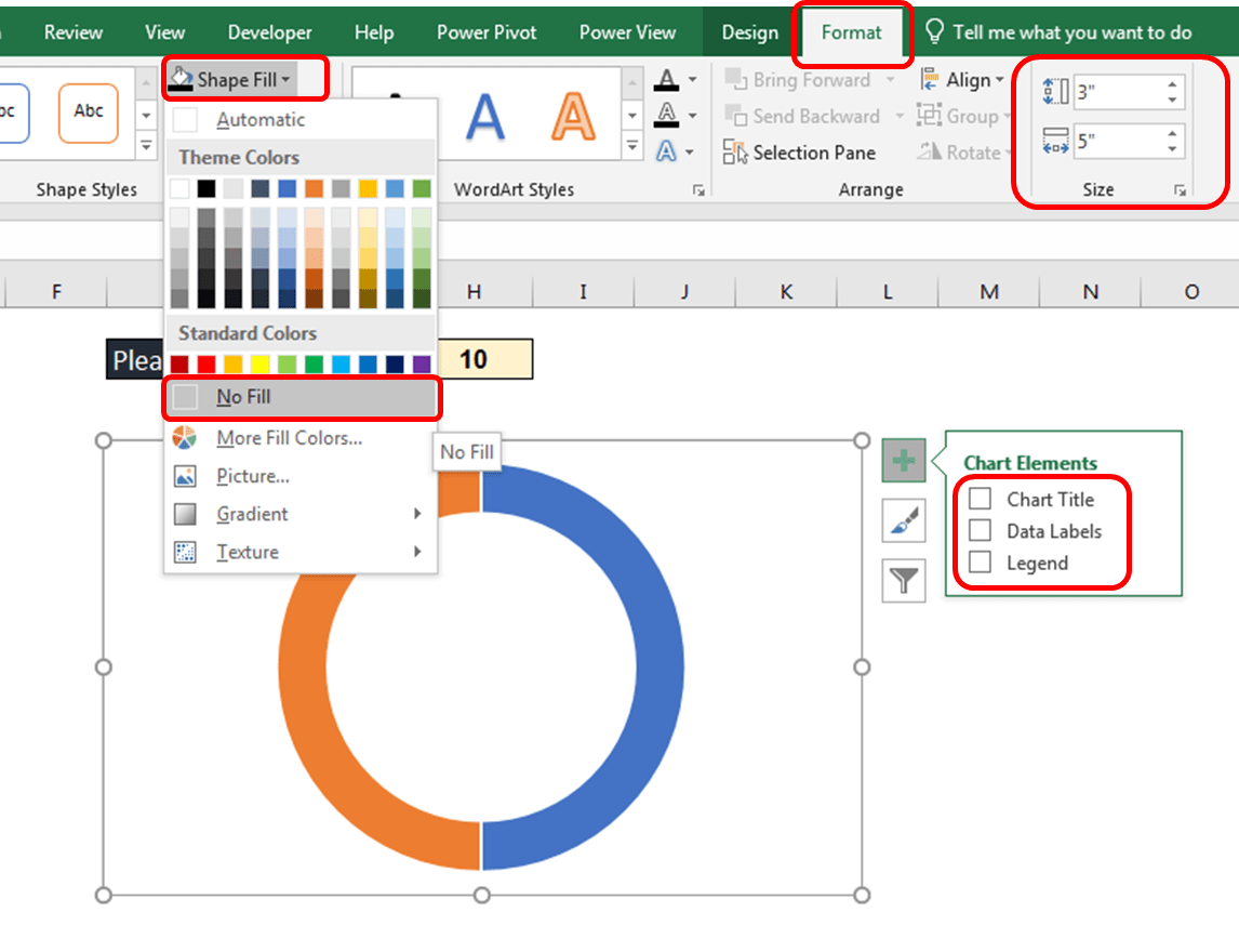
10.Select the Filled Axes (Blue color), go to Format Tab -> Click on Shape Fill -> More Fill Colors -> Click on Custom tab in Colors dialog box -> Enter the Color code as Red: 102; Green: 255; Blue:255. Now Click on OK.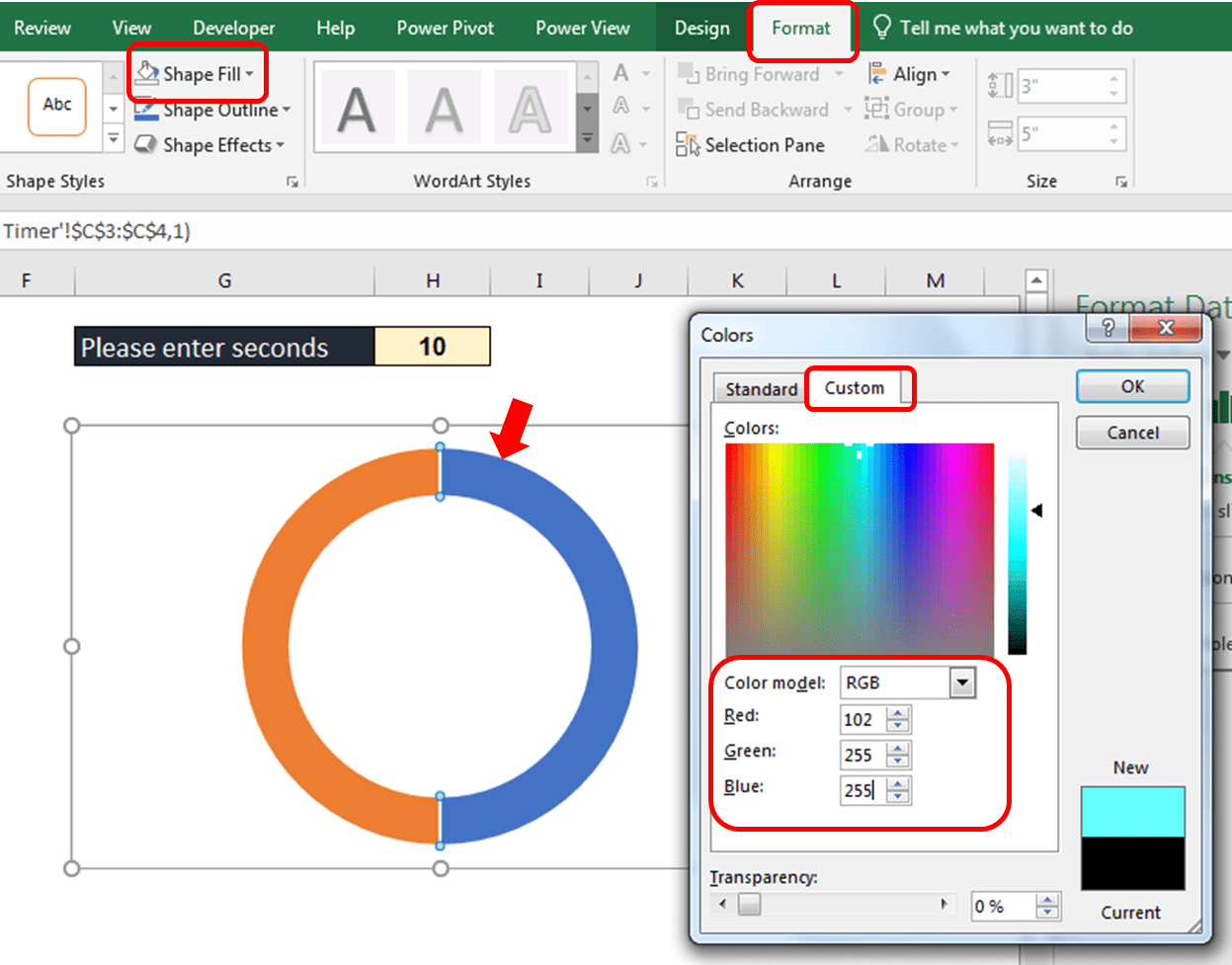
11.Select the ‘Not Filled’ Axes (Orange color), go to Format Tab -> Click on ‘Shape Fill’ -> Select ‘White Background 1, Darker5%’ and set the Transparency to 64% after click on ‘More Fill Colors…’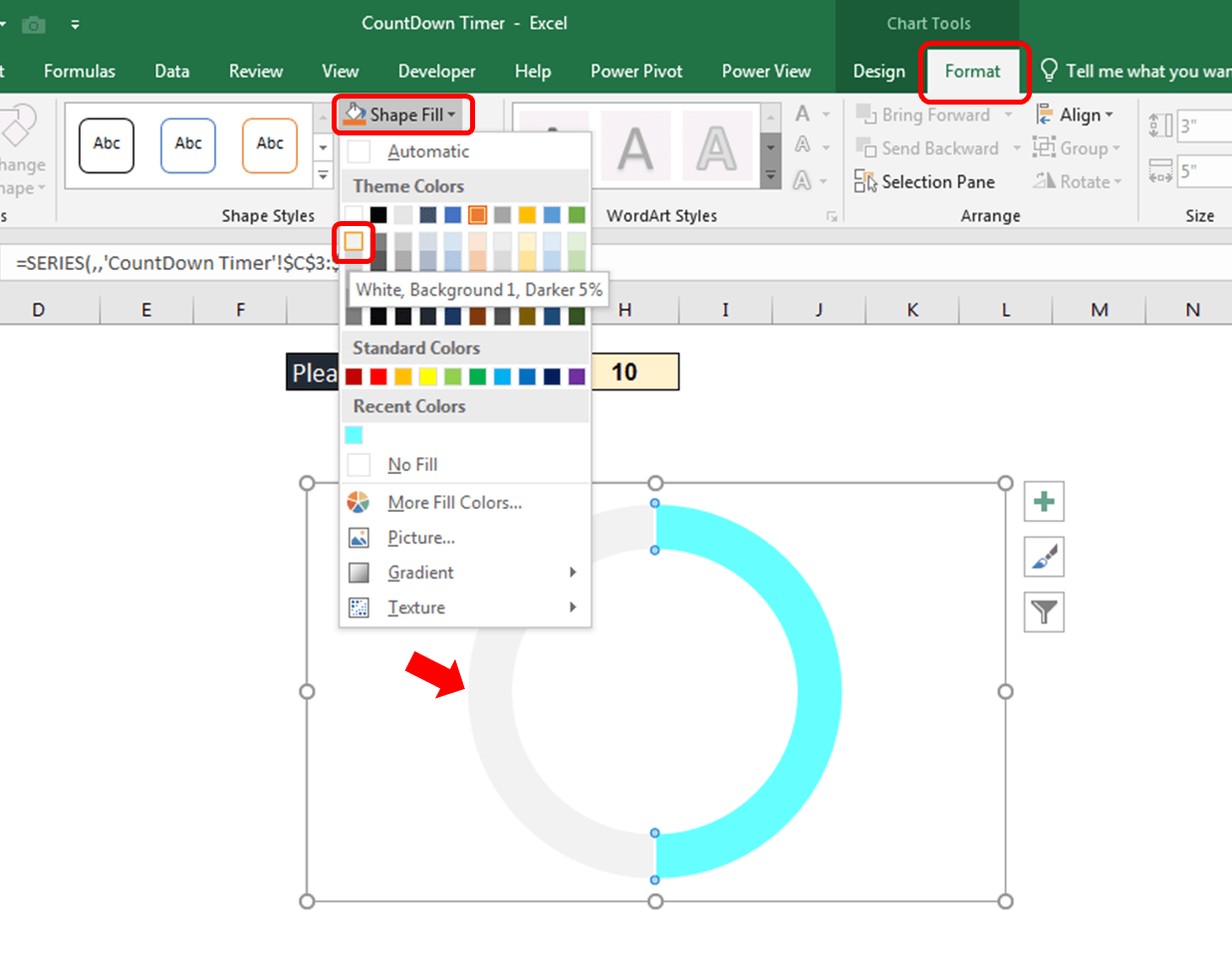
12.Right Click on Plot Area then ‘Click on Format Data Series…’. Go to ‘Format Data Series’ pane and change the ‘Doughnut Hole Size’ from 75% to 85%.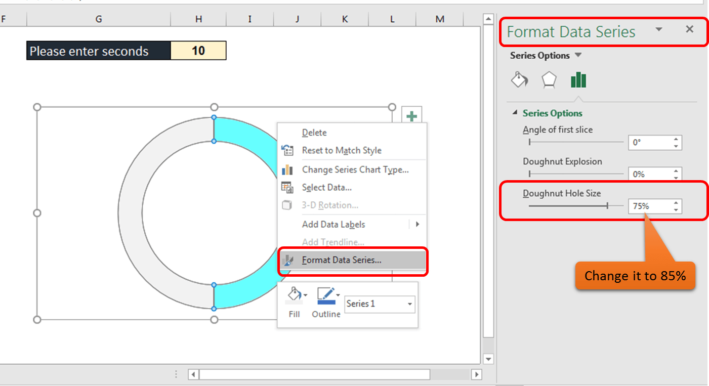
13.Select the Doughnut, go to Format Data Series and select ‘Border’ as ‘No Line’
14.Select the Range C7:C9 in Pie Chart table. Go to Insert tab, click on Pie Chart and select 2D Pie Chart
15.Select the Pie Chart, go to Format tab and change the Size: Width=5” and Height=3”. Click on + icon available at the top right corner of the chart and untick Chart Title, Data Labels and Legend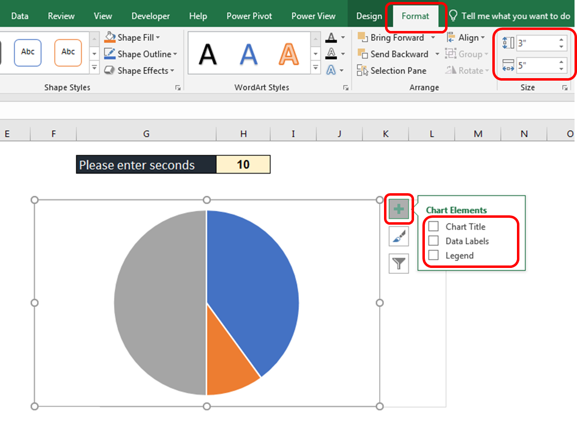
16.In this Pie Chart, we have three different slices are available. First one is ‘Not filled – 1’ (filled with blue color), second one is ‘Filled’ (filled with orange color) and third one is ‘Not filled – 2’ (filled with gray color). Let us change the color and formatting of each slice.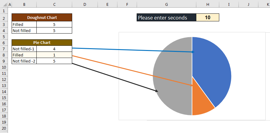
17.Select the Pie chart, got to Format tab then click on ‘Shape Outline’ and select ‘No Outline’ remove the lines available in Pie Chart.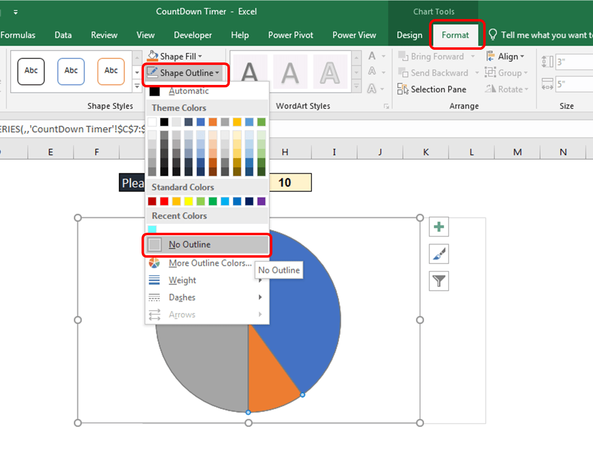
18.Select the First Slice (filled with blue color), right click on it then click on ‘Format Data Point…’, click on ‘Fill & Line’ icon in Format Data Point pane then select the ‘No fill’ option button. Repeat the same steps for Third Slice (filled with gray color).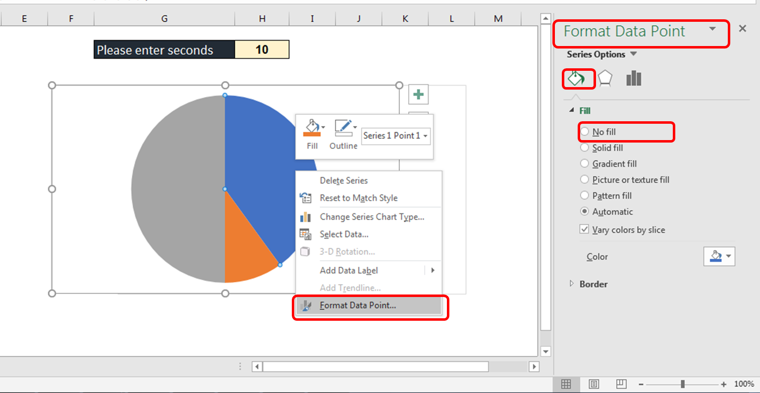
19.Post applying ‘No fill’ for first and third slices, chart will look like the below one. We will have only once slice visible (fill with orange color as of now)
20.Change the color and formatting of second slice as well.
21.Select the second slice, go to ‘Format Data Point’ pane, click on ‘Fill & Line’. Select ‘Gradient fill’ option, Type as ‘Linear’, Angle as 225 Create two different Gradient stops 1st at 0% and 2nd at 53%. Select the color of 1st gradient stop as Red- 102; Green- 255; Blue-255. Select the color of 2nd gradient stop as ‘White Background – 1’ and Transparency as 100%.
22.Now, select the chart, got to ‘Format Chart Area’ pane. Click on ‘Fill & Line’, select the ‘Solid fill’ option and select color as ‘Black’.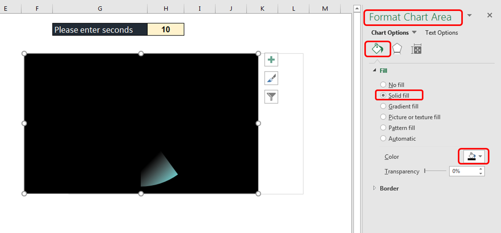
23.Now, right click on Chart and select ‘Send to Back’.
24.Select both the charts (Pie & Doughnut), click on Format tab then click on Align and select ‘Align Center’ & ‘Align middle’.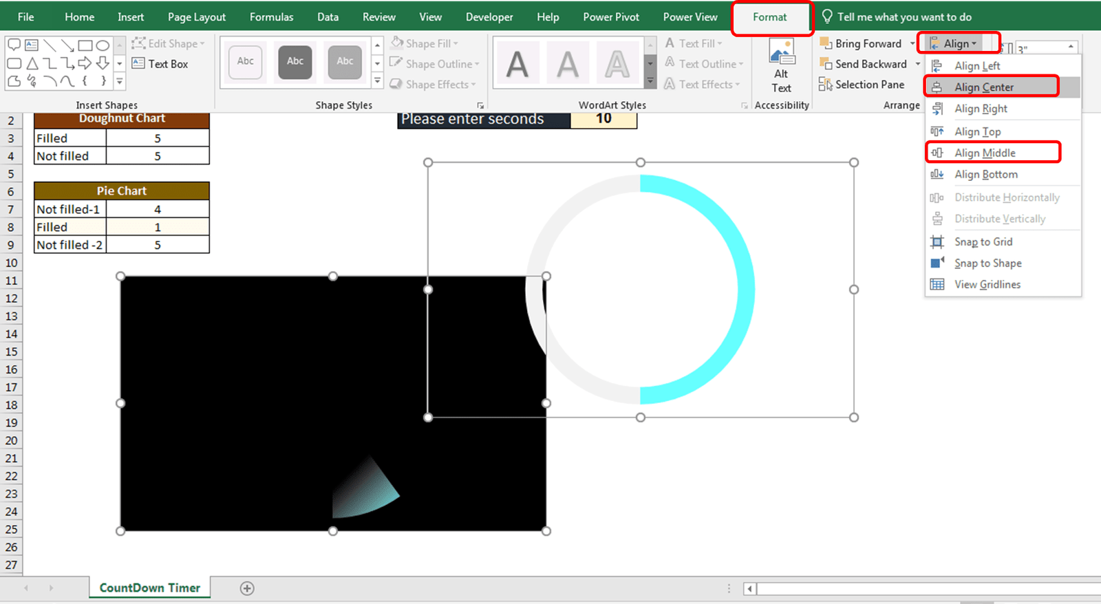
25.Now, insert a text box and give the reference of cell C4.
26.Select the text box, go to ‘Home’ tab. Change the font to ‘Calibri’, size to 80, Font color as ‘White’ and ‘Fill Color’ as ‘No Fill’.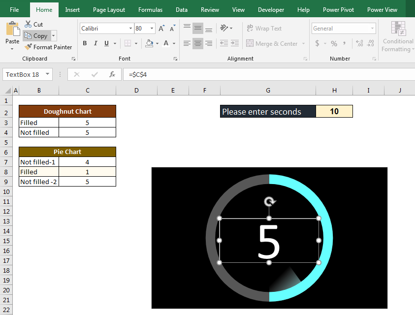
27.Select the text box, go to ‘Format’ tab then select ‘No Outline’ under shape styles group.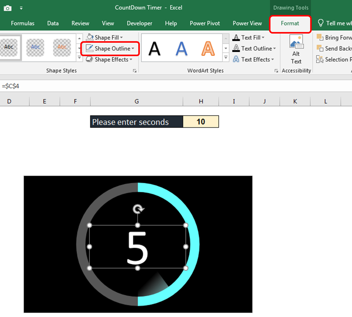
28.Enter the formulas in the first two highlighted tables (Doughnut Chart and Pie Chart). These formulas are required to add animation on this countdown timer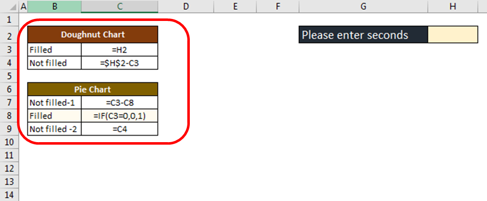
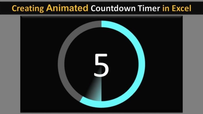
29.Select Pie Chart, Doughnut Chart and Text Box. Make all these objects aligned to center and middle. Move it and place below the cell ‘G2’. Now, Countdown time will look like below one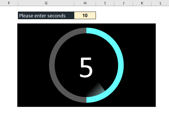
30.Go to VBE window, paste the below mentioned VBA Code to add animation under the Sheet1 code window.
Option Explicit Private Sub Worksheet_Change(ByVal Target As Range)
     If Target.Row = 2 And Target.Column = 8 Then
         Range("C3").Value = 0
         Dim CurrentTime
         Dim i As Integer
         Dim j As Integer
         j = Range("H2").Value
         For i = 1 To j
             CurrentTime = Timer
             Do While Timer < CurrentTime + 1
              DoEvents
             Loop
             Range("C3").Value = i
         Next i
     End If
 End Sub
Note: VBA Timer is an inbuilt function used to give us the fractional value of seconds. In above code, we are increasing the value of Cell C3 by one on every 1 second. To pause the code for 1 second, we are using Do While Loop and the condition is if Timer value is less than CurrentTime+1. If you want to convert the CountDown Timer from seconds to minutes then CurrentTime+1 would be replaced by CurrentTime+60 .
31.Switch to Excel and enter any value in cell ‘H2’ to check whether CountDown timer is working and animating as per our expectation or not.
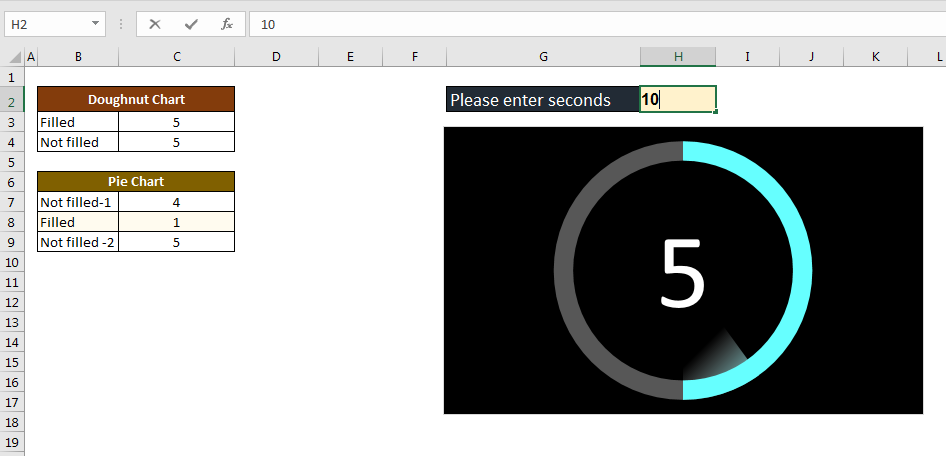
34. Now, Countdown timer tool is ready.
Please watch the complete tutorial on YouTube.
Click on download button to download the Excel file.




How can it used for minutes? at YT you wrote into the comments, that you will post a blog about it but i cant find it.
Thanks for your question! We have updated a not below the code in blog. Please check that. Hope, you will find useful in converting this to minutes.
How to increase the speed of the countdown?