Table of Contents
Introduction Magic Search Box in Excel
In the world of data management, Microsoft Excel stands as a versatile application, offering numerous tools and features to help users manipulate and analyze data. Yet, when working with large sets of records, finding specific information can be a difficult and time-consuming task. To make your life easier and more efficient, let’s unveil the magic of creating a search box in MS Excel. This nifty tool will transform the way you search and filter data within your spreadsheets.
Why Do You Need a Magic Search Box in Excel?
If you’ve ever spent valuable time scrolling through thousands or even millions of rows in an Excel spreadsheet, searching for a specific record containing the required piece of information, you’ll appreciate the need for a search box. A well-implemented search box can significantly boost your productivity, save time and minimize errors in your data query tasks. Plus, it’s incredibly easy to set up as you don’t need to use a single line of VBA code.
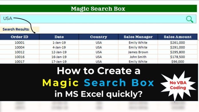
Watch the YouTube tutorial to create Magic Search Box in Excel
Creating the Magic Search Box in Excel
To create a magic search box in Excel, follow these simple steps:
Get Your Data Ready
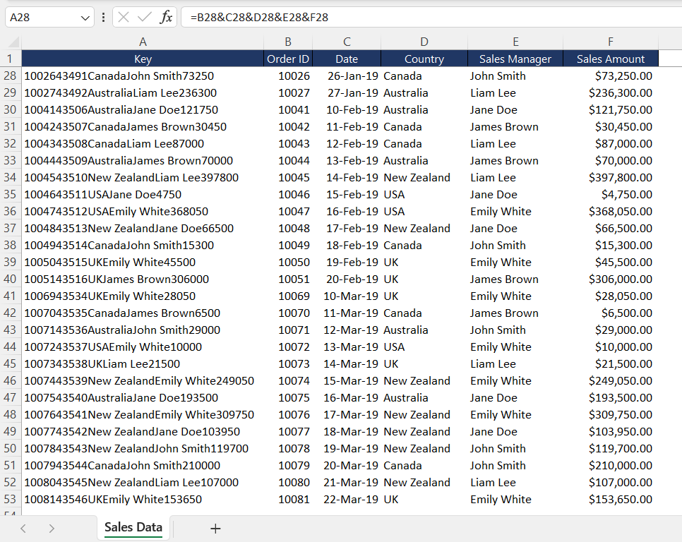
Start by creating a new worksheet in your Excel workbook and rename it to ‘Sales Data’. Now, copy and paste all your sales data into this new sheet, making sure you have all the necessary columns and records. Next, add a new column at the beginning of your sales table and name it “Key”. To fill this column with concatenated values of all the columns, use a formula to combine all the cell values in a row using the ampersand (&) symbol.
Creating Magic Search Box in Excel Interface
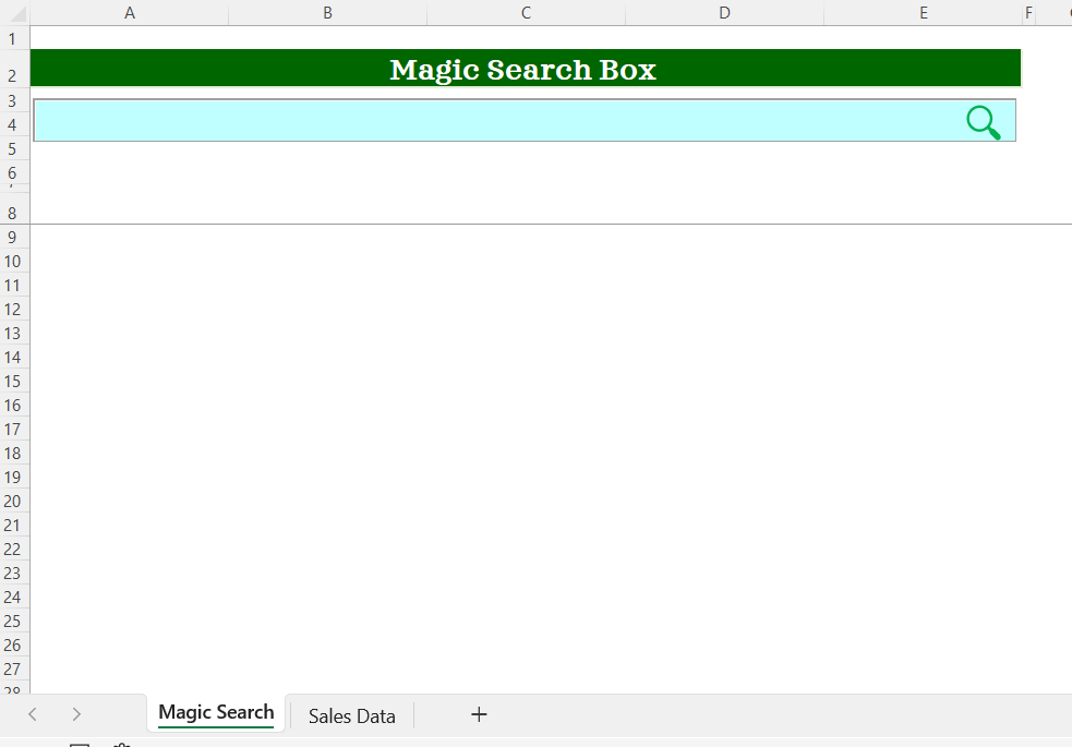
Start by adding a new sheet to your Excel workbook and rename it to ‘Magic Search.’ Now, let’s make it look nice and functional. Create a heading at the top and call it ‘Magic Search Box.’ You can make it eye-catching by coloring the background green and the text white or any other colors you prefer.
Right under this heading, you’ll want to add the actual search box. To do this, go to the ‘Developer’ tab, find the ‘Controls’ group, and click on ‘Insert.’ From there, choose the ‘Text Box’ option under ‘ActiveX Controls.’
Now, draw the text box right below the heading on your sheet. After you’ve got it in place, right-click on the text box and choose ‘Properties.’
In the properties window, you’ll see a spot labeled ‘Linked Cell.’ Here, type ‘A4.’ This step connects the search box to cell A4, so anything you type in the search box will also show up in cell A4. This link helps in searching and filtering data easily.
When you’ve got your linked cell set, click ‘Design Mode’ in the Developer tab to exit the design mode.
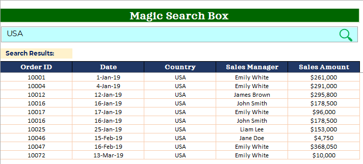
Create Headers and Enter Formulas to show the search result
First, you need to copy the headers (excluding ‘Key’) from the ‘Sales Data’ sheet and paste them into cell A8 on the ‘Magic Search’ sheet. Make these headers stand out by making them bold and formatting them nicely.
Above these column headers, in cell A6, type ‘Search Results.’
Now, let’s get to the formula part. In cell A9, put this formula:
=IFERROR(IF(A4="","",FILTER('Sales Data'!$B$2:$F$53,ISNUMBER(SEARCH(A4,'Sales Data'!$A$2:$A$53)))), "No Value Found").This formula works like this: It checks if cell A4 (which is linked to your search box) has a value. If it’s blank, it shows nothing as a search result. If there’s something in A4, it uses the Filter function to go through the data in ‘Sales Data’ (from B2 to F53).
To filter the data, it uses the Search function. This function looks for the value in A4 within the range A2 to A53 in the ‘Sales Data’ sheet. If it finds a match, it gives a number as the output. If not, it shows an error (#Value).
The ISNUMBER function helps by deciding if the result is true or false, and this info is passed to the Filter function. If there’s an error at any step, the IFERROR function steps in to display ‘No Value Found’ as the result.
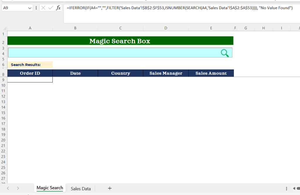
Now, we are done with creating the Magic Search Box in Excel.
Download the demo file of Magic Search Box in Excel.


