Develop Live Currency Converter in Excel
MS Excel–based live currency converter is a simple and easy‑to‑use tool that converts currency from one exchange to another. You don’t need to download any additional application or visit a website. Excel retrieves the currency data from a forex website (any website you choose while developing the tool) and keeps refreshing the data at a set interval.
In this post, we are going to learn how to develop a fully automated real‑time currency converter in Microsoft Excel. Using Power Query, we will extract live currency data from the website freeforexapi.com and convert the data into the required format for the Currency Converter tool. You can apply the same logic to retrieve data from any forex website and connect it to your Excel‑based utility tool.
If you are interested in developing this utility tool, you can follow the steps mentioned below. If you prefer to skip the development for now, you can download the sample tool using the download button available at the end of this post. Happy learning!
Creating Excel File and Connecting to forex website
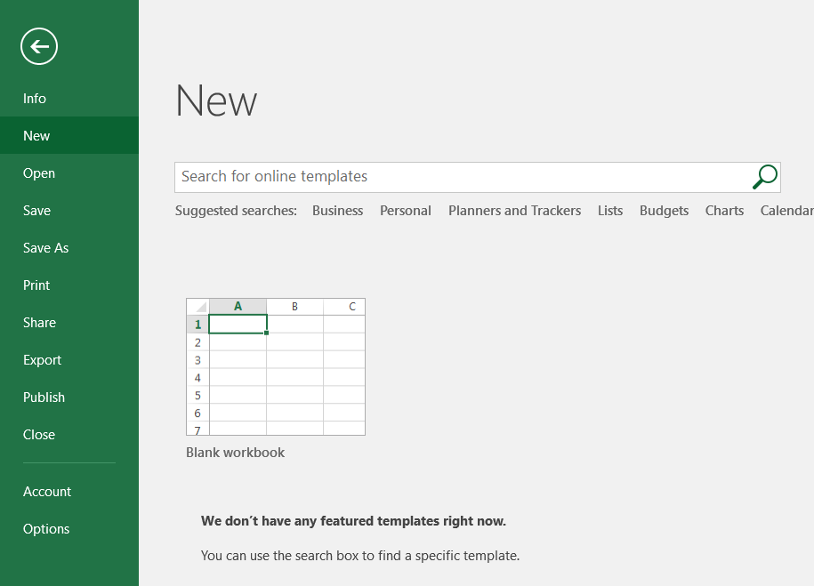
1. Open Microsoft Excel Application and create a new blank workbook.
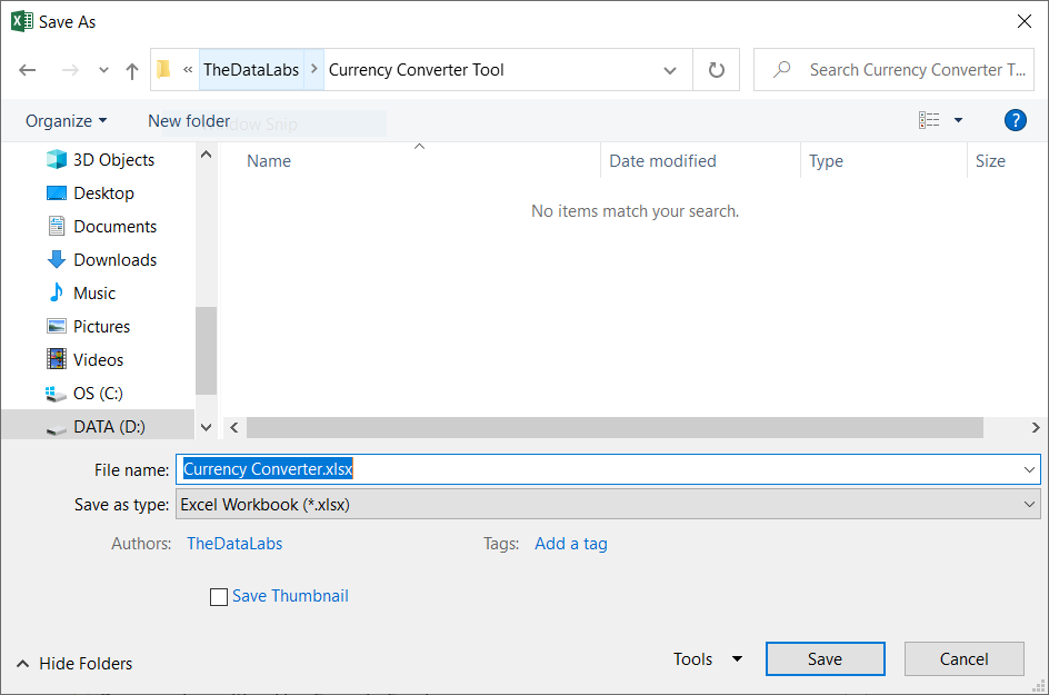
2. Save the file with the name ‘Currency Converter’ with extension .xlsx.
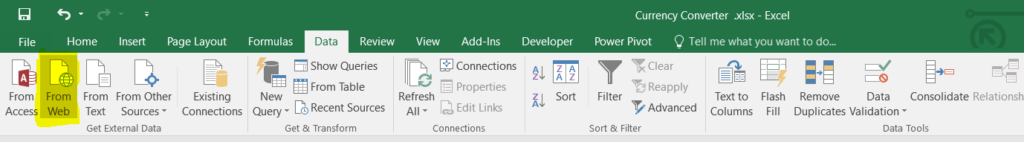
3. Click on Data Tab and under ‘Get External Data‘ group, click on ‘From Web‘ icon to connect and get the data from website.
4. In New Web Query window, enter the website name https://www.freeforexapi.com/ in Address field and then click on Import button to load and show the data in New Web Query window.
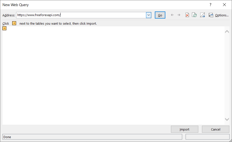
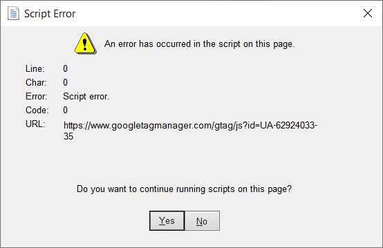
If you see any script error while importing the data, click on the Yes button to run the script on the page. It may ask for the same confirmation several times so that it can successfully connect with the given website and load the data into the New Web Query window.
Once you see all the details in the New Web Query window, click on the Import button again to import the data from the website into the Excel worksheet.
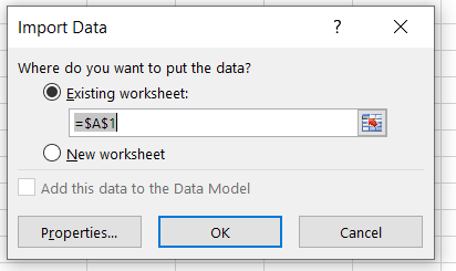
5. Select the Existing Worksheet option and provide a cell address, or choose the New Worksheet option in the Import Data window to import the data into the Excel worksheet. We will set the properties later.
You can see the imported raw data from the given website in a sheet. This is a single‑column table available in Column A.
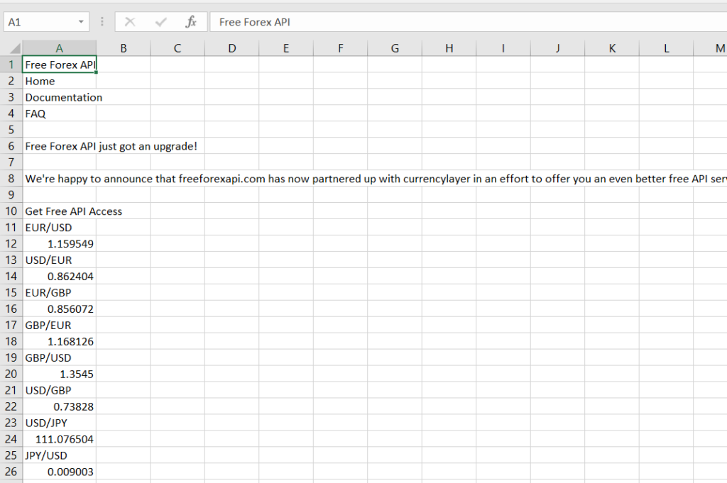
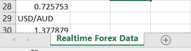
6. Rename the sheet from Sheet1 to Realtime Forex Data.
Cleaning & Processing Data in Power Query
Now, we need to load the data into Power Query so that we can remove unwanted rows, clean the data, and create the required columns for our use.
Follow the steps below to clean the data in Power Query.
1. First of all, we need to load the data into Power Query. To do this, place your cursor on any cell in Column A, click on the Data tab, and then click on From Table under the Get & Transform group.
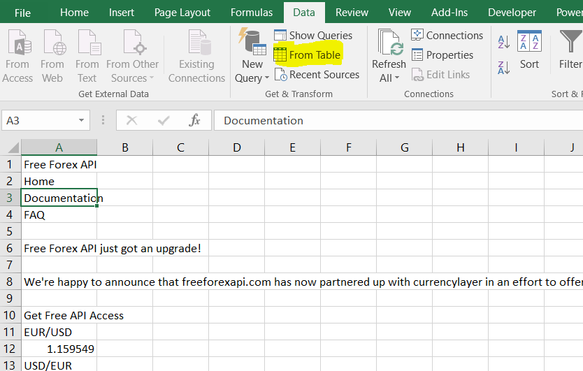
Once you click on the From Table button, it will load the table available in Column A and open the Power Query window. You can see the image below.
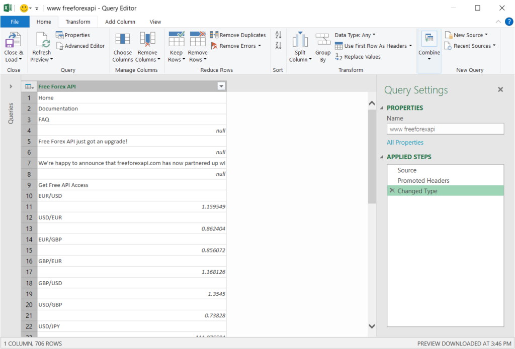
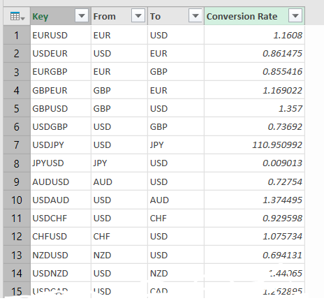
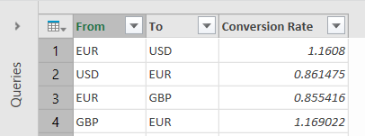
Currently, the data has been loaded into Power Query in a purely raw format. We need to clean this data and convert it into the format shown below.
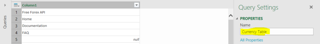
2. Let’s convert the raw data as shown in the snapshot above. First, we need to change the name of the query from www.freeforexapi.com to Currency Table.
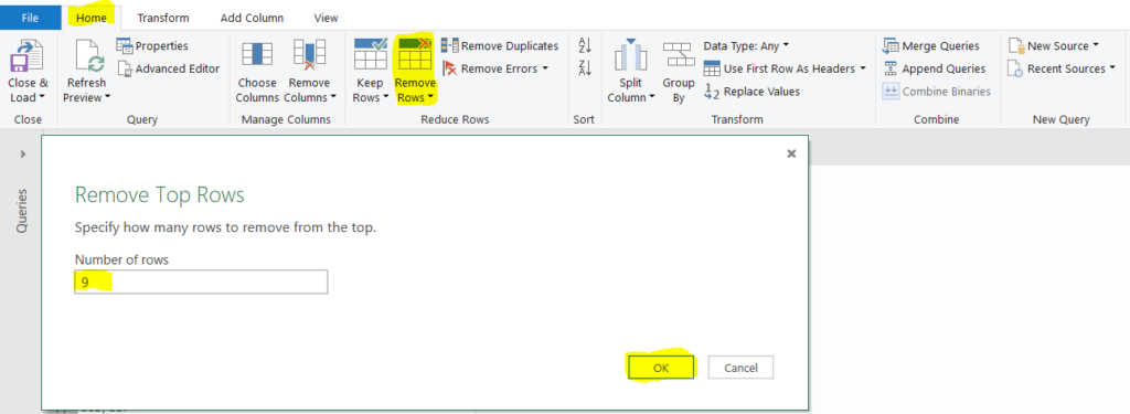
3. Now, we need to remove unwanted rows from the Currency Table. If you look at the table closely, you can see that the rows starting from 1 to 9 are unwanted, and we don’t need them.
To remove the top 9 rows, click on the Home tab in Power Query, then click on the Remove Rows button, and select the first option from the drop‑down menu, i.e., Remove Top Rows. A new window will open where you can enter the total number of rows to remove from the top of the table. Enter 9 and then click on the OK button.
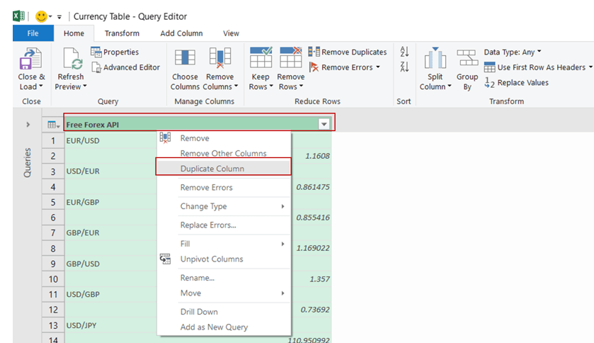
4. As this table has only one column containing the currency name and currency value, we need to separate them into two different columns. To do this, we first need to create a duplicate of the existing column for further processing.
To make a duplicate column, right‑click on the column header and then select Duplicate Column from the pop‑up menu (as shown in the snapshot below).
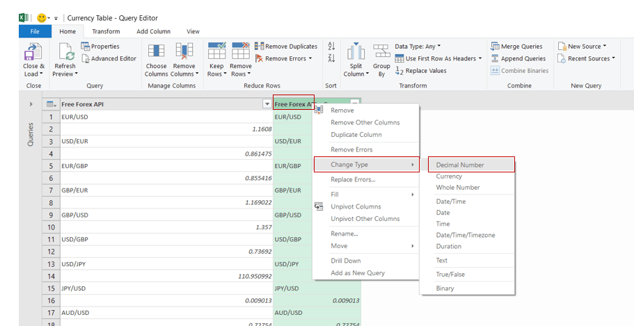
5. Now, you can see two columns in the table. Let’s convert the data type of the second column to Decimal Number. To do this, right‑click on the second column header, then click on Change Type, and select Decimal Number.
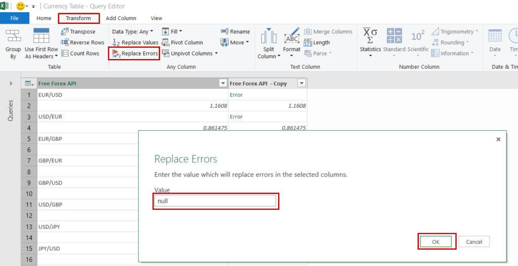
6. After converting the data type of the second column to Decimal Number, you can see that all the text values have been converted into error values. We need to replace these error values with null.
To replace the error values with null, click on the Transform tab, then click on the Replace Errors button. A new window will open where you can enter the value as null and then click on OK. This will replace all the error values with null in the second column.
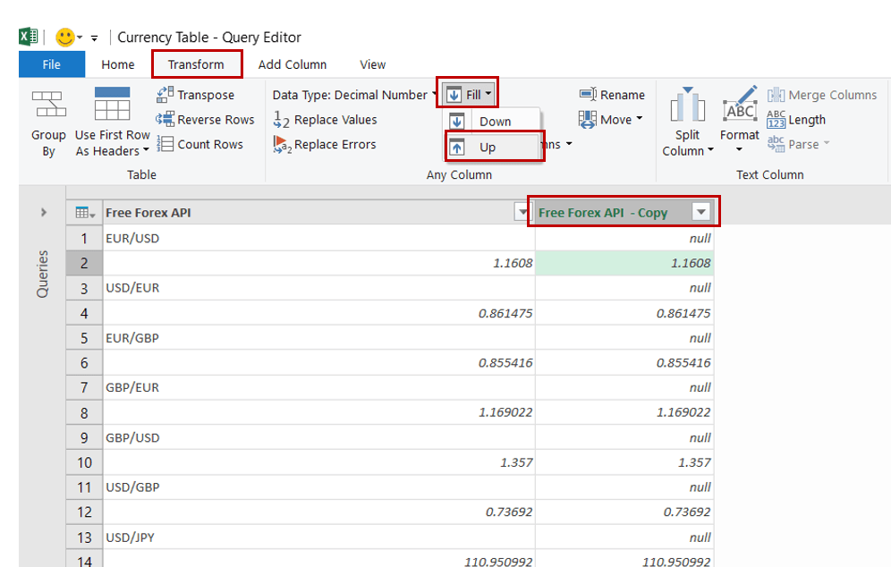
7. Now, we need to update the currency values against the row numbers where the currency names are available. Currently, null is displayed next to each currency name. To fill these null values with the corresponding currency values, we can use the Fill Up feature.
To use the Fill Up feature, select the header of the second column, then click on the Transform tab. Next, click on the Fill drop‑down menu and choose Up from the options. All the null values will be replaced by the numbers available below.
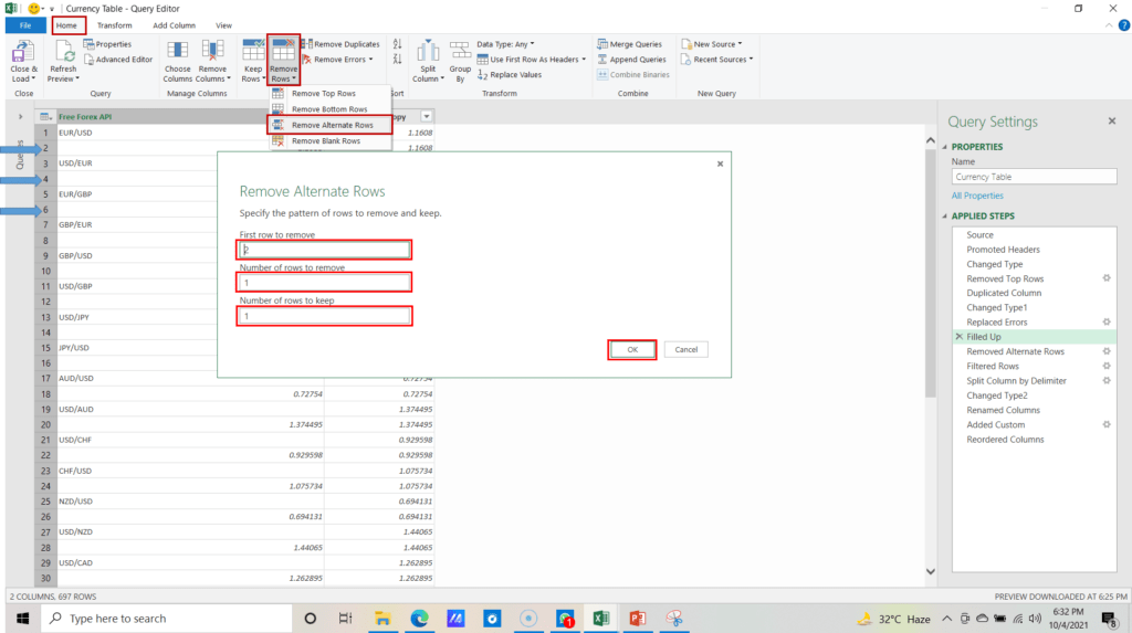
8. Now, you can see that every alternate row in the first column is blank. To clean the table, we need to remove these alternate rows.
To remove alternate rows from the table, click on the Home tab, then click on Remove Rows, and from the drop‑down options select Remove Alternate Rows. A window will open where you need to provide three inputs: First row to remove, Number of rows to remove, and Number of rows to keep. Please see the descriptions of these input fields below.
- First row to remove – Enter the row number(index or position) that you want to remove or you want to skip from.
- Number of rows to remove – Enter the number of rows you want to remove each time.
- Number of rows to keep – Enter the number of rows you want to keep.
Enter 2, 1, and 1 respectively as we need to start removing the record from Row Number 2 and then remove 1 row each time and keep 1 row after that. After entering the required row numbers, click on OK to process the request.
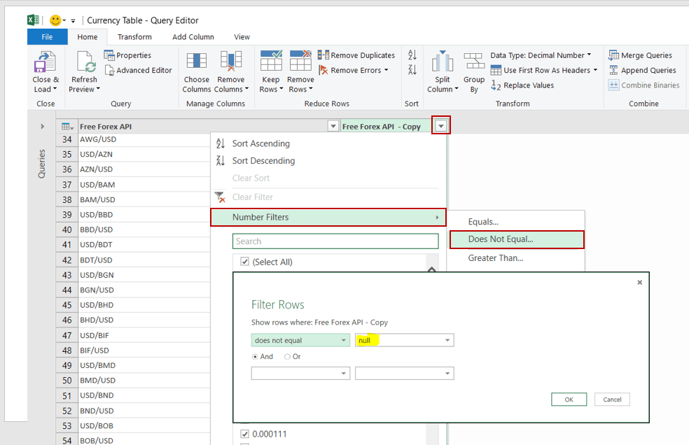
9. If you go to the end of the table, you can see null values appearing in the last rows of the second column. We need to remove these rows where null values are present.
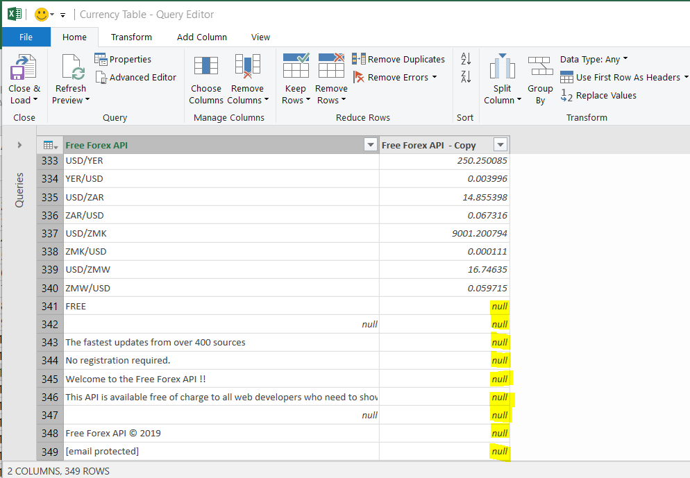
To filter the rows containing null values, click on the drop‑down button in the header of the second column, then click on Number Filters → Does Not Equal…. This will open the Filter Rows window. Enter null in the input field for the first filter option (Does Not Equal) and then click on OK. The table will now be filtered to remove all rows with null values in the second column.
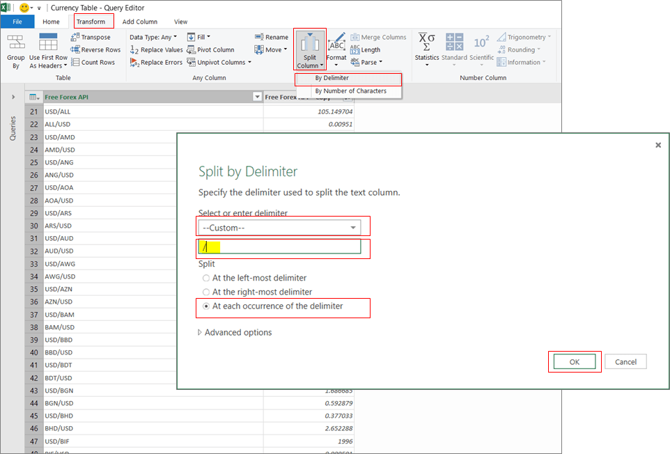
10. Now, we need to split the first column value by the delimiter e.g. /. It will help us in converting first column into two columns From Currency Name and To Currency Name.
To split the column, click on the header of the first column and then select the Transform tab, click on Split Column drop-down and select By Delimiter. It will open a new window where you need to select –Custom– from the first drop-down (select or enter delimiter), then enter back slash (/) in next input field, select At each occurrence of the the delimiter from the Split Options and then click on OK.
Once you will click on OK button then it will split the first column into two columns as shown in below snapshot.
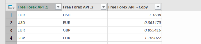
11. Now, we need to rename the header of all these three columns. Rename the column name from ‘Free Forex API.1‘ to ‘From‘, ‘Free Forex API.2‘ to ‘To‘ and ‘Free Forex API – Copy‘ to ‘Conversion Rate‘.
To rename the columns, just right click on the first column header and then enter the required name. Repeat the same activity for rest of the columns.
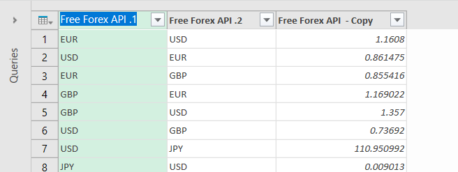
Once, you will rename all these columns then headers name will be as shown in below image.
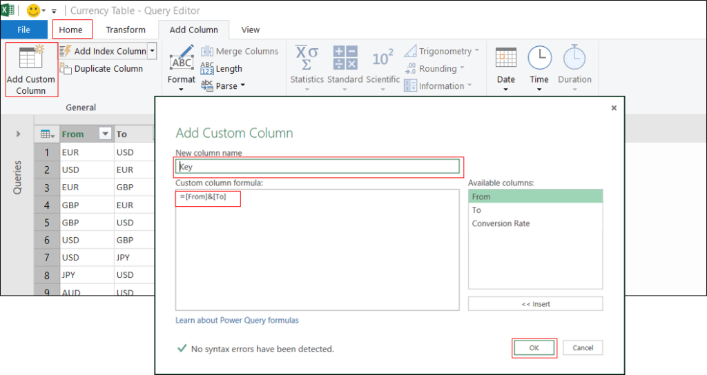
12. Now, we need to create a custom column “Key”. It will help us to lookup the currency conversion rate in MS Excel when user will convert the currency from one exchange to another.
To add a custom column, just click on Home tab then click on Add Custom Column button in General group. It will open a new window ‘Add Custom Column‘. Here, you need to provide the inputs for ‘New column name‘ & ‘Custom column formula‘. New column name would be ‘Key‘ and formula would be ‘[From]&[To]‘. After entering the required inputs, just click on OK button.
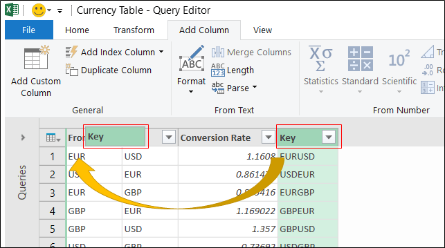
Once, we will click on OK button then it will insert the Key column to the extreme right of the table. Here, we need to move the newly added column from the right side of table to the beginning of the table.
To move the column, just click on column header and while holding the mouse button, move the column to the left side of the table and release the mouse button (it’s like drag and drop). See the below image.
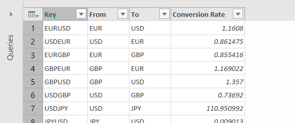
Once, you complete the movement of column, your table will look like below image.
13. Now, we need one additional table with a single column i.e. ‘Currency Name’. This column will be utilized to create drop-down for ‘From’ and ‘To’ currency name field.
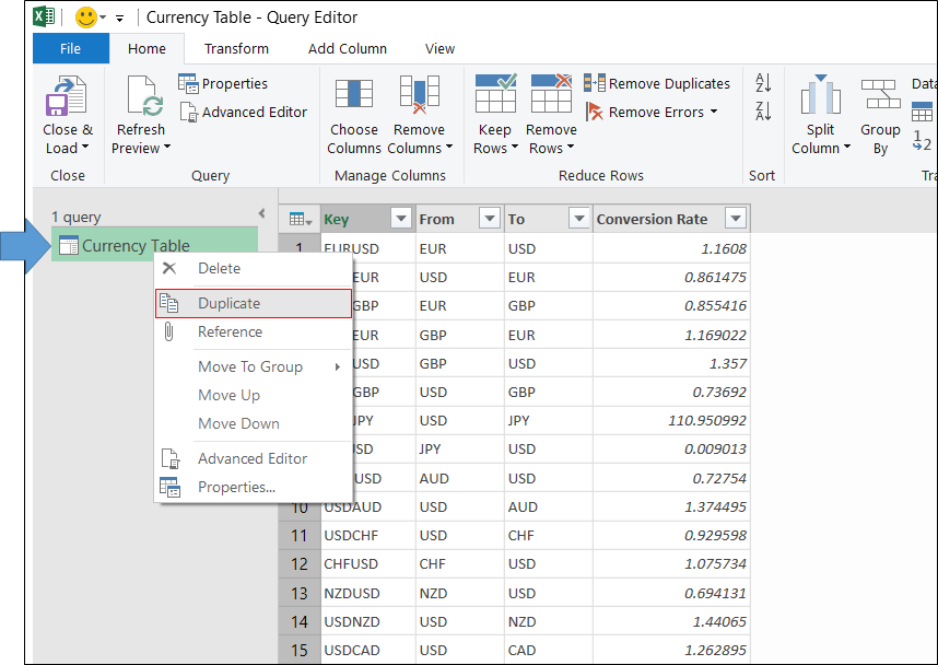
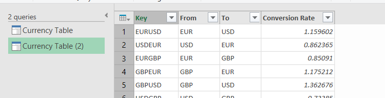
To create the new table, we will utilize the duplicate table features of Power Query. Right click on ‘Currency Table‘ in query section and then click on ‘Duplicate‘. It will create a duplicate copy of the Currency Table with the name Currency Table (2).
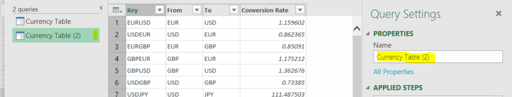
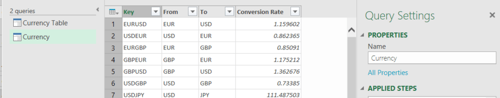
14. Rename the duplicate table from Currency Table (2) to Currency. To do that, just click on ‘Currency Table (2)’ in query section and provide the new name under the properties of Query section. Enter the name ‘Currency’. I
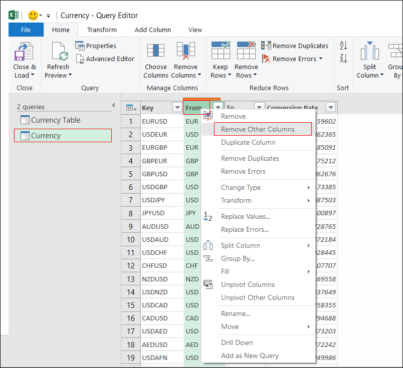
15. Now, we need to remove the unwanted columns from the Currency table and keep only one column having currency name value.
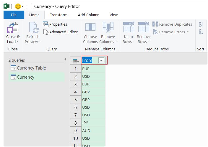
To remove the extra columns, just select the Currency in query pane and then right click on the column header ‘From’. From pop-up menu, click on Remove Other Columns. It will remove all the other columns and keep From column only in this table.
16. Rename the column header from ‘From’ to ‘Currency Name’. To do that, just double click on the column header and then rename the column header to Currency Name.
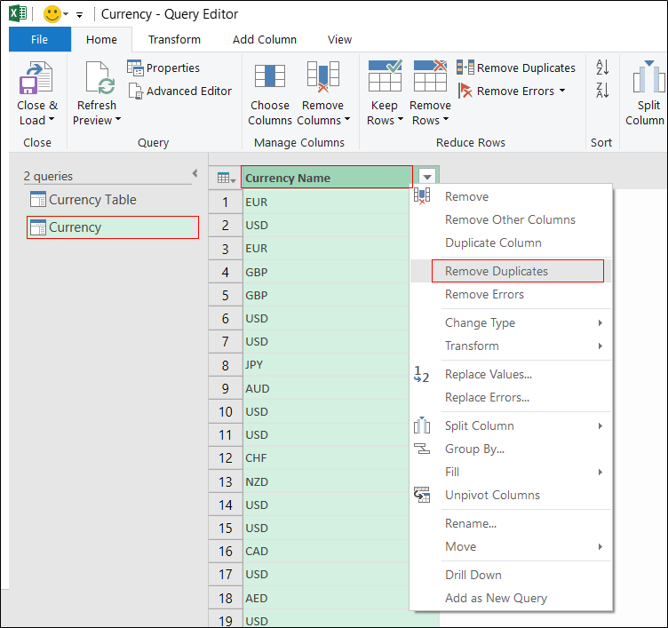
17. If you closely observe the column, you can see duplicate currency name/code are reflecting. We need to remove all the duplicates value and keep unique in this colulmn.
To remove the duplicates, right click on Currency Name column and then select the Remove Duplicates from the pop-up menu. It will delete all the duplicate values available in column.
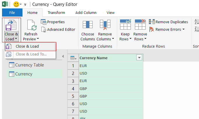
18. Now, we have done with data cleaning and processing. Let’s load the data to Excel Sheet. To do that, just move to Home tab and then click on Close & Load button and select Close & Load under Query group. It will load both the table Currency Table and Currency in two separate worksheets.
Creating Name and Designing User Interface for Currency Converter
1. Let’s move to Excel file and select Currency worksheet. In this sheet, you can see a one column table which has all the available currency name/code. We need to define a Name in Excel so that we can utilize it while creating drop-down fields in Currency Converter User Interface.
To create a dynamic name, just press shortcut key CTRL + F2. It will open Name Manager window. In Name Manager, just click on New… button to create a new name.
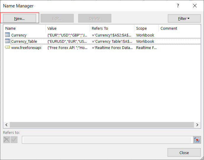
It will open New Name window where you can define Name and provide the Refers To: value. In Name input box, enter Currency_Name and then in Refers to: field, enter to formula to select complete range of currency name starting from row 2 to end. This formula will keep adjusting the range basis on data availability. Use the below formula and then click on OK button. It will create a new name called Currency_Name.
=OFFSET(Currency[[#Headers],[Currency Name]],1,0,COUNTA('Currency'!$A:$A),1)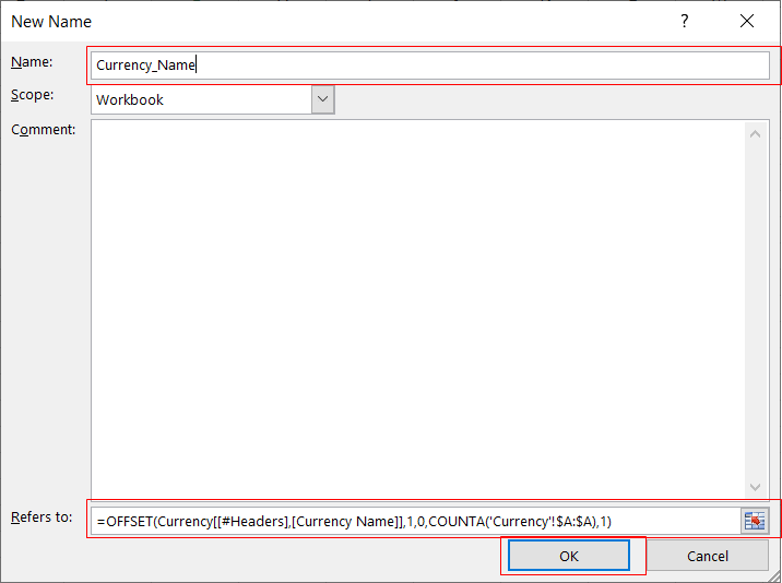
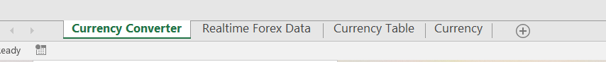
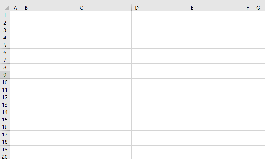
2. Now, we need to design the User Interface of Currency converter. To do that, just insert a blank worksheet and rename it to Currency Converter.
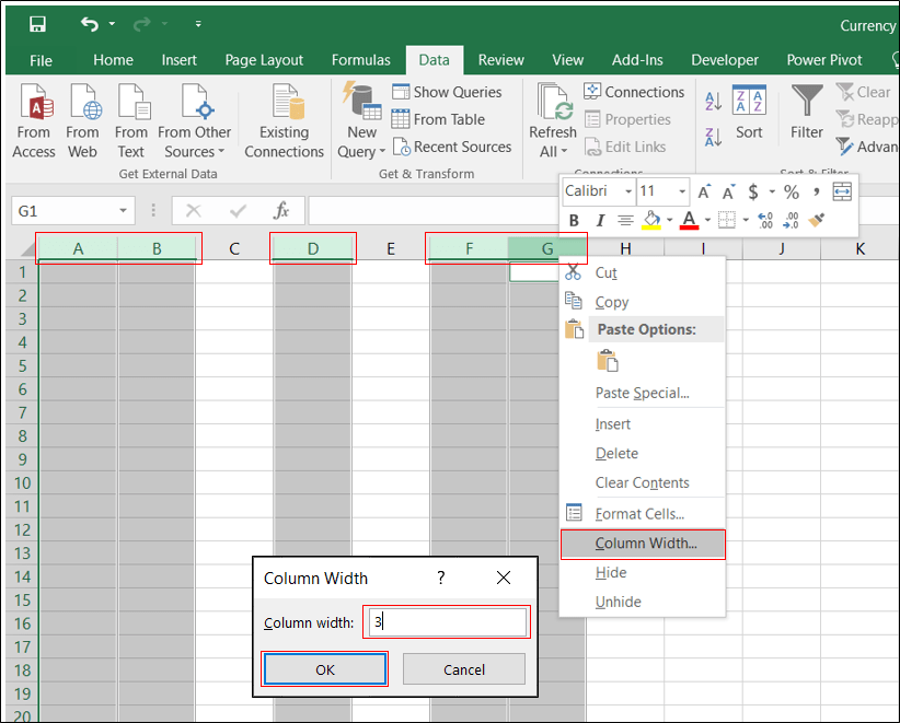
3. Select columns A, B, D, F and G with mouse click while holding CTRL Key. After selecting the columns, right click on header and then click on Column Width…. It will open a pop-up window for Column Width. Enter the column width as 3 and then click on OK button.
4. Follow the above step to set the column width of C and E. Width should be 35. Once you set the columns width, your Excel sheet will look like the below snapshot.
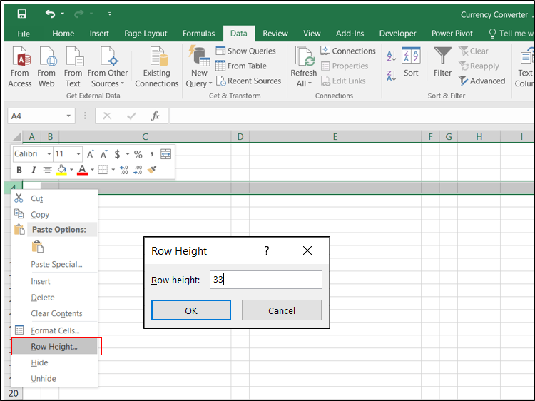
5. Set the height of row number 4. To do that just right click on the header of Row 4 then click on Row Height…. In Row Height pop-up window, provide the height as 33 and then click on OK button.
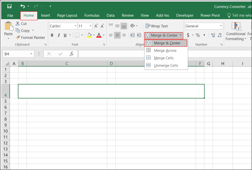
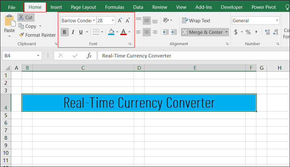
6. Merge the range B4:F4. To do that, just select the cell starting from B4 to F4 and click on Home tab then click on Merge & Center.
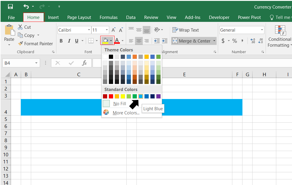
7. Fill the merged cell with light blue color. To do that, just select the merged cells (B4:F4) and click on Home tab then click on Fill color bucket and click on Light blue color in color palettes.
8. Enter the header in merged cell as ‘Real-Time Currency Converter’ using Font name, Barlow Condensed Thin, Font Size – 28 and Font formatting – Bold. You can select the font name, size and style Font group in Home tab.
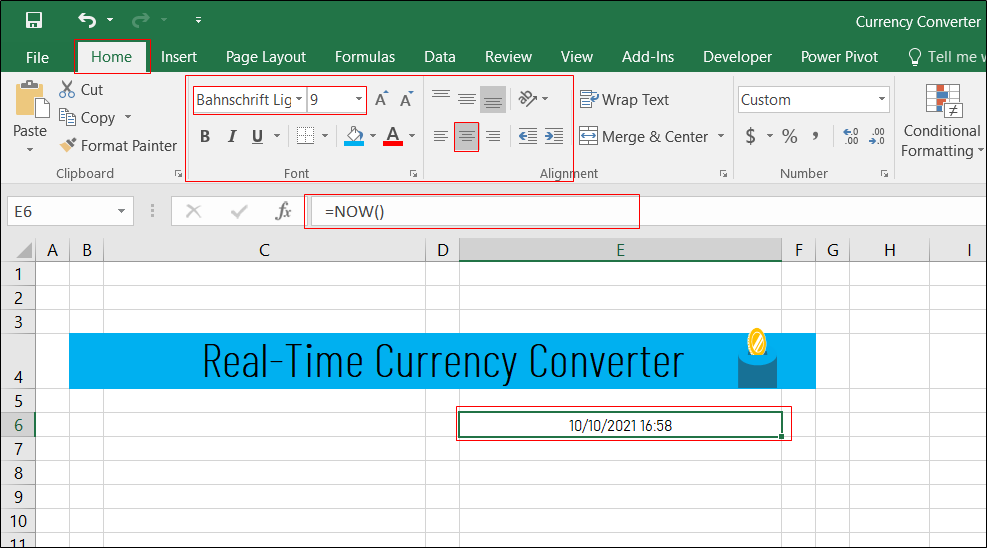
9. Copy the icon which you have planned to use in Currency converter and then paste it to the right side of header (or as per your design).

10. Select the cell E6 and then enter the formula =Now(). Go to Home tab and select the font Bahnschrift Light, font size 9 and alignment Center.
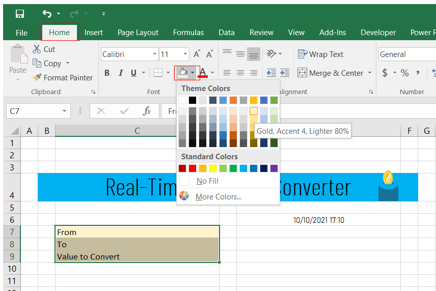
11. Enter ‘From‘ in cell C7, ‘To‘ in cell C8 and ‘Value to Convert‘ in cell C9. Select the range starting from C7 to C9 and then click on Home tab and choose the fill color as Gold, Accent 4, Lighter 80%. Now, merge the cells C7 & D7, C8 & D8 and C9 & D9.
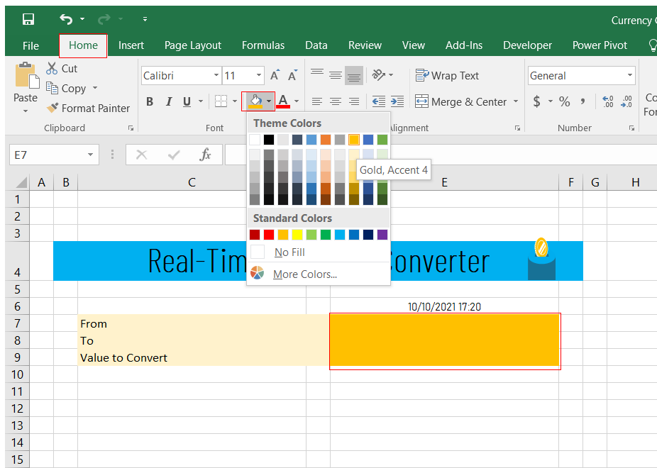
12. Select the cells E7 to E9 then click on Home tab and select Gold, Accent 4 as fill color.
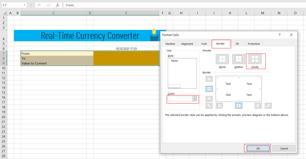
13. Now, apply the border with white color on C7:E9. To do that, just select the range C7:E9 and then press shortcut key as CTRL + 1. In Format Cells window, click on Border and select style as simple line, color as white, click on Inside and then click on OK to apply the border.
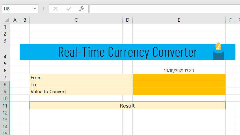
14. Select the cells C11 to E11 and enter the text header as ‘Result‘ and fill color as Gold, Accent 4, Lighter 80%. Apply border with simple line and color as Light Blue.
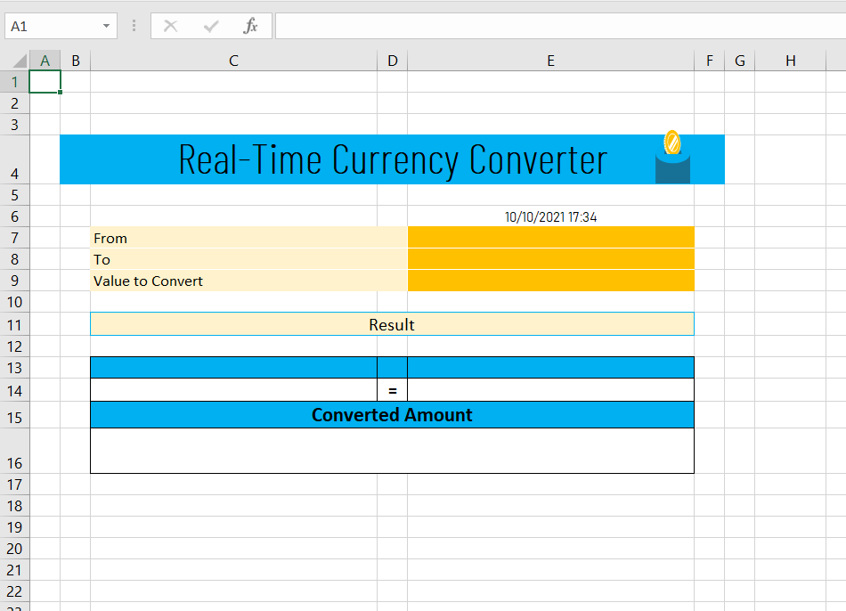
15. Fill the cells C13, D13 and E13 with Light Blue color. Enter equal sign (=) in cell D14. Merge the range C15 to E15 and enter the text as ‘Converted Amount‘ with Font face Bold. Enter Row height as 31 for row number 16. Apply black color border on the range C13:E16.
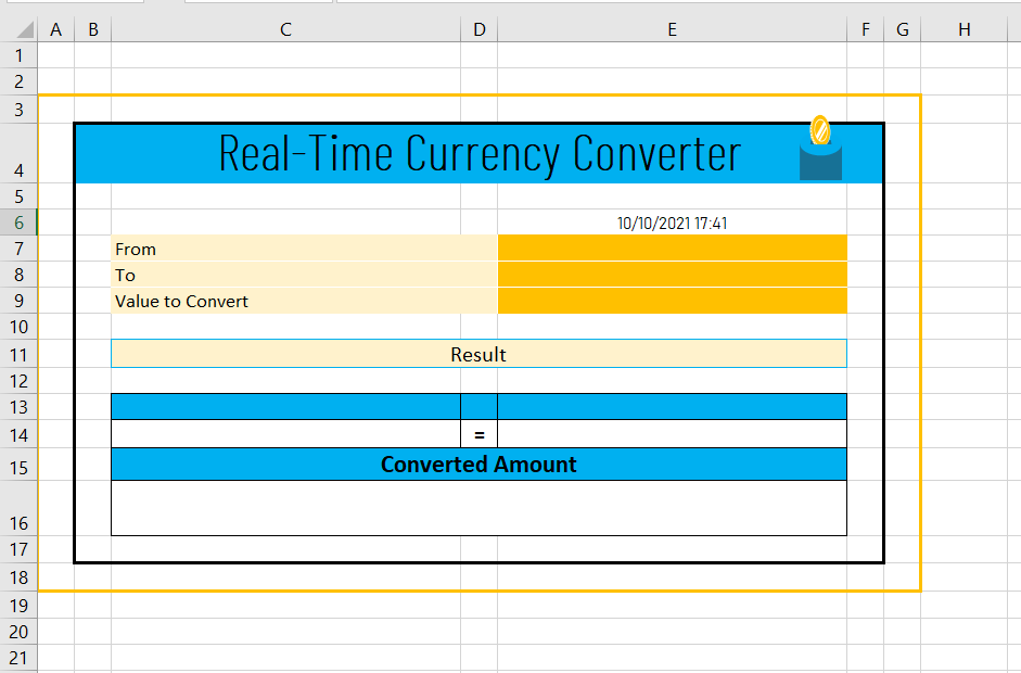
16. Apply 5 as row height for row number 12. Also, apply black and gold color border as shown in below image.
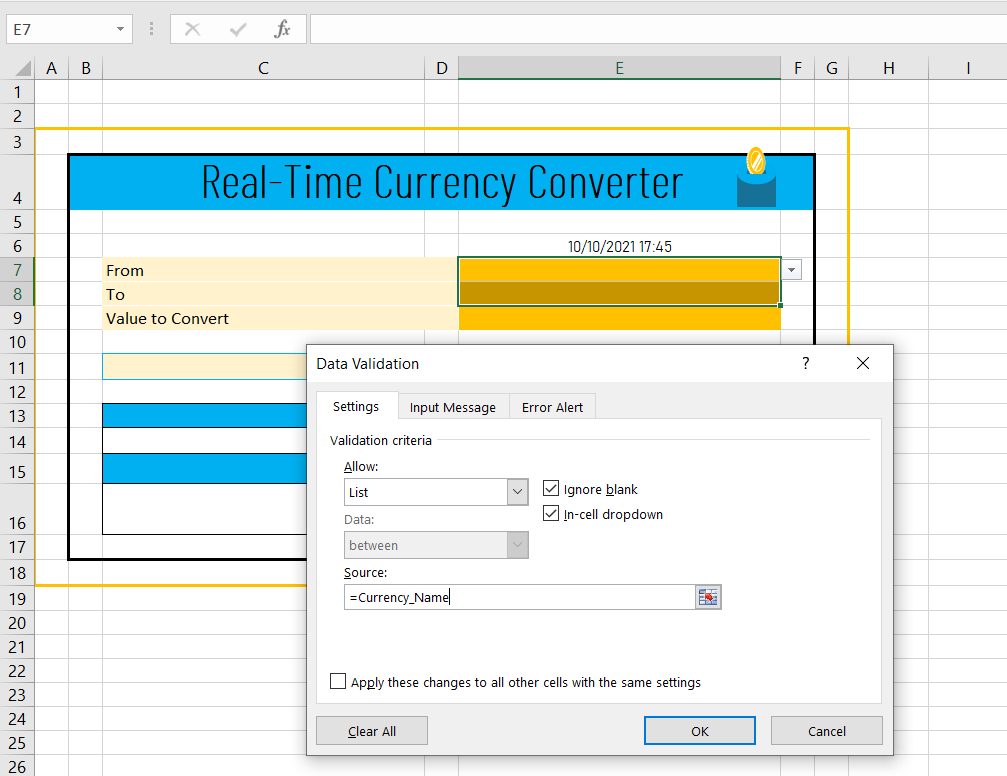
17. Let’s create a drop-down fields for From and To. To do that, just select cells E7 & E8 and then press shortcut key ALD + D + L to open the Data Validation window.
In Data Validation window, click on Setting tab then select List from Allow drop-down and in Source: field, enter the name which we have created for currency name i.e. Currency_Name with preceding equal sign (=) as show in below image. Once, you enter the name then click on OK button. It will create drop-down fields for both From and To.
18. Hide the row number 1 & 2 and some other rows and columns which are not required. Also, remove the gridlines from the worksheet.
Enter the formula in C13 to refer the selected currency name from ‘From‘ field. In E13, give the reference of currency name available in ‘To‘. Apply the formula to lookup the currency value based on Key from Currency table. Enter the formula in cell C14 so that it can validate whether From and To currency name are same or not. If both are same then the currency value would be the same which is available in E14 and if not then it would be 1. Apply formula to multiply the given amount in Value to convert (E9) with the currency value available in E14.
List of formulas:
C13 -> =$E$7
E13 -> =$E$8
C14 -> =IF(E8=””,””,1)
E14 -> =IFERROR(IFERROR(VLOOKUP($E$8&$E$9,’Currency Table’!$A:$D,4,0),VLOOKUP($E$8&”USD”,’Currency Table’!$A:$D,4,0)*VLOOKUP(“USD”&$E$9,’Currency Table’!$A:$D,4,0)),””)
C16 -> =IFERROR($E$10*$E$15,””)
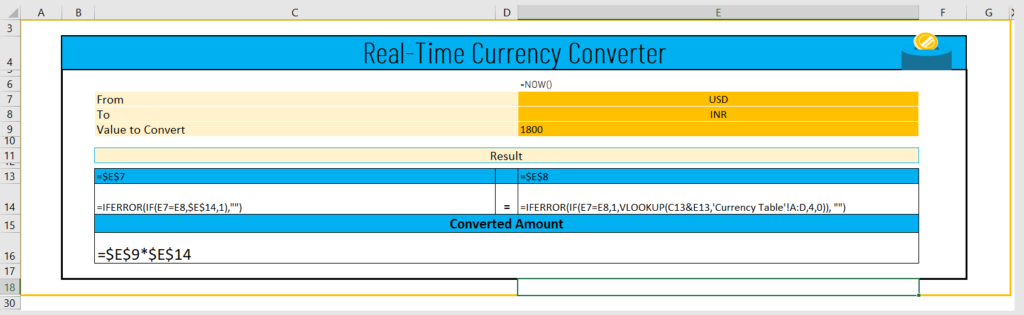
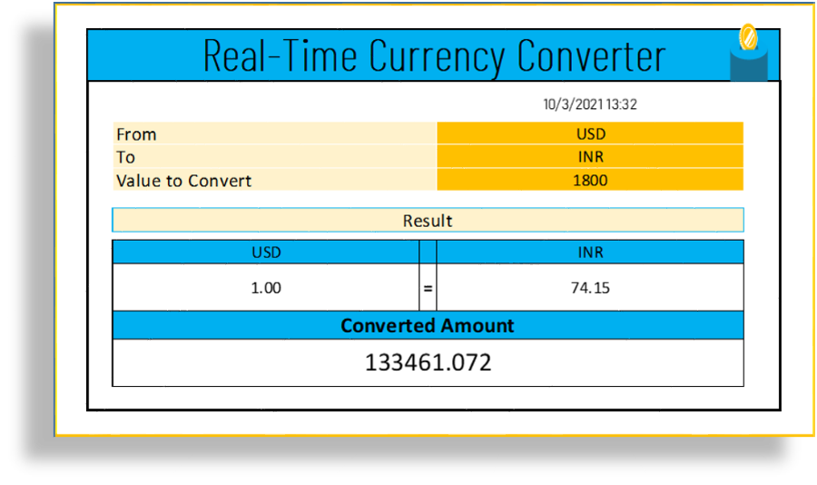
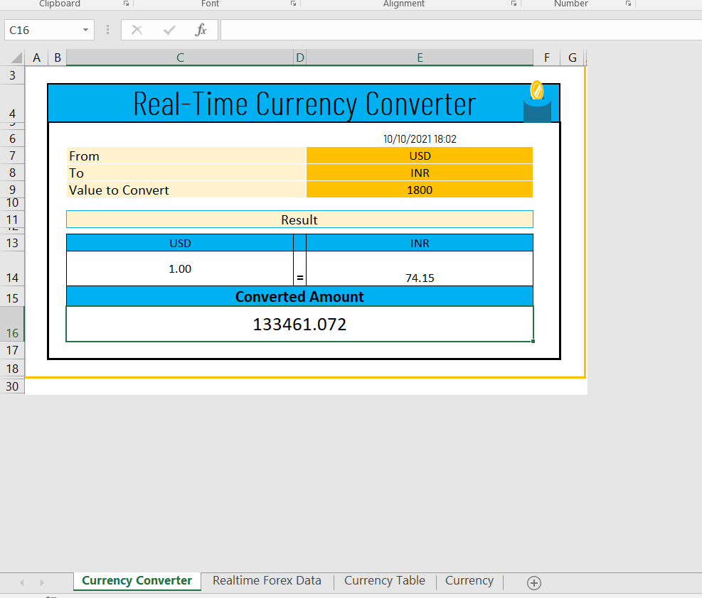
19. Once you done with entering the formulas, your currency converter will look like as show in below image. You can see the converted value of 1800 USD is available in Cell C16.
Set the refresh frequency
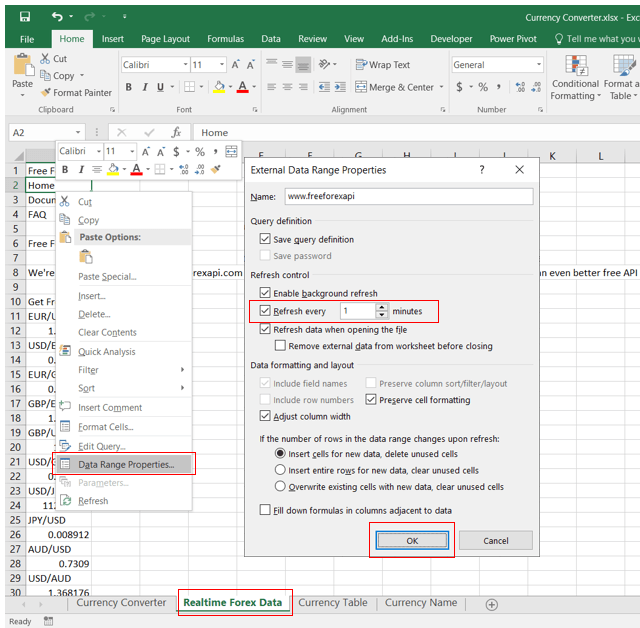
To set the refresh frequency of forex data, just move to Realtime Forex Data sheet, right click on any of the cell in Column A and from pop-up menu, select Data Range Properties… . It will open External Data Range Properties window where you can set several properties. Here, we need to focus only on Refresh every field. Just provide 1 as input so that it can refresh the data on every 1 minute. You can set the time as per your requirement tool. After input the time, click on OK.
This is all about creating a Currency Converter with the help of Excel and Power Query. If you have any question or feedback, please leave a comment below. We will go though the comment and reply as soon as possible. Thanks!
Please watch YouTube tutorial – Develop Live Currency Converter in Excel
Download
Please download the sample file for Develop Live Currency Converter in Excel by clicking on the button below.

Disclaimer: This post is only for educational purpose. We have used the website https://www.freeforexapi.com/ to extract the forex data that is only for demo purpose to show how can we connect and import the data from a website. TheDataLabs team is not responsible for any type of errors, delay in data refreshing or data discrepancies and licensing issue.


